This article is the 7th part of a series about named table expressions. In Part 5 and Part 6 I covered the conceptual aspects of common table expressions (CTEs). This month and next my focus turns to optimization considerations of CTEs.
I’ll start by quickly revisiting the unnesting concept of named table expressions and demonstrate its applicability to CTEs. I’ll then turn my focus to persistency considerations. I’ll talk about persistency aspects of recursive and nonrecursive CTEs. I’ll explain when it makes sense to stick to CTEs versus when it actually makes more sense to work with temporary tables.
In my examples I’ll continue using the sample databases TSQLV5 and PerformanceV5. You can find the script that creates and populates TSQLV5 here , and its ER diagram here. You can find the script that creates and populates PerformanceV5 here.
Substitution/unnesting
In Part 4 of the series, which focused on optimization of derived tables, I described a process of unnesting/substitution of table expressions. I explained that when SQL Server optimizes a query involving derived tables, it applies transformation rules to the initial tree of logical operators produced by the parser, possibly shifting things around across what were originally table expression boundaries. This happens to a degree that when you compare a plan for a query using derived tables with a plan for a query that goes directly against the underlying base tables where you applied the unnesting logic yourself, they look the same. I also described a technique to prevent unnesting using the TOP filter with a very large number of rows as input. I demonstrated a couple of cases where this technique was quite handy—one where the goal was to avoid errors and another for optimization reasons.
The TL;DR version of substitution/unnesting of CTEs is that the process is the same as it is with derived tables. If you’re happy with this statement, you can feel free to skip this section and jump straight to the next section about Persistency. You won’t miss anything important that you haven’t read before. However, if you’re like me, you probably want proof that that’s indeed the case. Then, you will probably want to continue reading this section and test the code that I use as I revisit key unnesting examples that I previously demonstrated with derived tables and convert them to use CTEs.
In Part 4 I demonstrated the following query (we’ll call it Query 1):
USE TSQLV5;

  SELECT orderid, orderdate
  FROM ( SELECT *
     FROM ( SELECT *
            FROM ( SELECT *
                   FROM Sales.Orders
                   WHERE orderdate >= '20180101' ) AS D1
            WHERE orderdate >= '20180201' ) AS D2
     WHERE orderdate >= '20180301' ) AS D3
  WHERE orderdate >= '20180401';
The query involves three nesting levels of derived tables, plus an outer query. Each level filters a different range of order dates. The plan for Query 1 is shown in Figure 1.
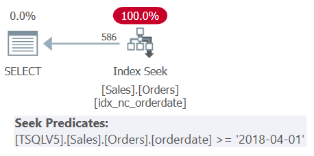 Figure 1: Execution plan for Query 1
The plan in Figure 1 clearly shows that unnesting of the derived tables took place since all filter predicates where merged into a single encompassing filter predicate.
I explained that you can prevent the unnesting process by using a meaningful TOP filter (as opposed to TOP 100 PERCENT) with a very large number of rows as input, as the following query shows (we’ll call it Query 2):
  SELECT orderid, orderdate
  FROM ( SELECT TOP (9223372036854775807) *
     FROM ( SELECT TOP (9223372036854775807) *
            FROM ( SELECT TOP (9223372036854775807) *
                   FROM Sales.Orders
                   WHERE orderdate >= '20180101' ) AS D1
            WHERE orderdate >= '20180201' ) AS D2
     WHERE orderdate >= '20180301' ) AS D3
  WHERE orderdate >= '20180401';
The plan for Query 2 is shown in Figure 2.
 Figure 2: Execution plan for Query 2
The plan clearly shows that unnesting did not take place as you can effectively see the derived table boundaries.
Let’s try the same examples using CTEs. Here’s Query 1 converted to use CTEs:
  WITH C1 AS
  (
    SELECT *
    FROM Sales.Orders
    WHERE orderdate >= '20180101'
  ),
  C2 AS
  (
    SELECT *
    FROM C1
    WHERE orderdate >= '20180201'
  ),
  C3 AS
  (
    SELECT *
    FROM C2
    WHERE orderdate >= '20180301'
  )
  SELECT orderid, orderdate
  FROM C3
  WHERE orderdate >= '20180401';
You get the exact same plan shown earlier in Figure 1, where you can see that unnesting took place.
Here’s Query 2 converted to use CTEs:
  WITH C1 AS
  (
    SELECT TOP (9223372036854775807) *
    FROM Sales.Orders
    WHERE orderdate >= '20180101'
  ),
  C2 AS
  (
    SELECT TOP (9223372036854775807) *
    FROM C1
    WHERE orderdate >= '20180201'
  ),
  C3 AS
  (
    SELECT TOP (9223372036854775807) *
    FROM C2
    WHERE orderdate >= '20180301'
  )
  SELECT orderid, orderdate
  FROM C3
  WHERE orderdate >= '20180401';
You get the same plan as shown earlier in Figure 2, where you can see that unnesting did not take place.
Next, let’s revisit the two examples that I used to demonstrate the practicality of the technique to prevent unnesting—only this time using CTEs.
Let’s start with the erroneous query. The following query attempts to return order lines with a discount that is greater than the minimum discount, and where the reciprocal of the discount is greater than 10:
  SELECT orderid, productid, discount
  FROM Sales.OrderDetails
  WHERE discount > (SELECT MIN(discount) FROM Sales.OrderDetails)
  AND 1.0 / discount > 10.0;
The minimum discount cannot be negative, rather is either zero or higher. So, you’re probably thinking that if a row has a zero discount, the first predicate should evaluate to false, and that a short circuit should prevent the attempt to evaluate the second predicate, thus avoiding an error. However, when you run this code you do get a divide by zero error:
  Msg 8134, Level 16, State 1, Line 99
  Divide by zero error encountered.
The issue is that even though SQL Server does support a short circuit concept at the physical processing level, there’s no assurance that it will evaluate the filter predicates in written order from left to right. A common attempt to avoid such errors is to use a named table expression that handles the part of the filtering logic that you want to be evaluated first, and have the outer query handle the filtering logic that you want to be evaluated second. Here’s the attempted solution using a CTE:
  WITH C AS
  (
    SELECT *
    FROM Sales.OrderDetails
    WHERE discount > (SELECT MIN(discount) FROM Sales.OrderDetails)
  )
  SELECT orderid, productid, discount
  FROM C
  WHERE 1.0 / discount > 10.0;
Unfortunately, though, the unnesting of the table expression results in a logical equivalent to the original solution query, and when you try to run this code you get a divide by zero error again:
  Msg 8134, Level 16, State 1, Line 108
  Divide by zero error encountered.
Using our trick with the TOP filter in the inner query, you prevent the unnesting of the table expression, like so:
  WITH C AS
  (
    SELECT TOP (9223372036854775807) *
    FROM Sales.OrderDetails
    WHERE discount > (SELECT MIN(discount) FROM Sales.OrderDetails)
  )
  SELECT orderid, productid, discount
  FROM C
  WHERE 1.0 / discount > 10.0;
This time the code runs successfully without any errors.
Let’s proceed to the example where you use the technique to prevent unnesting for optimization reasons. The following code returns only shippers with a maximum order date that is on or after January 1st, 2018:
  USE PerformanceV5;

  WITH C AS
  (
    SELECT S.shipperid,
      (SELECT MAX(O.orderdate)
       FROM dbo.Orders AS O
       WHERE O.shipperid = S.shipperid) AS maxod
    FROM dbo.Shippers AS S
  )
  SELECT shipperid, maxod
  FROM C
  WHERE maxod >= '20180101';
If you’re wondering why not use a much simpler solution with a grouped query and a HAVING filter, it has to do with the density of the shipperid column. The Orders table has 1,000,000 orders, and the shipments of those orders were handled by five shippers, meaning that in average, each shipper handled 20% of the orders. The plan for a grouped query computing the maximum order date per shipper would scan all 1,000,000 rows, resulting in thousands of page reads. Indeed, if you highlight just the CTE’s inner query (we’ll call it Query 3) computing the maximum order date per shipper and check its execution plan, you will get the plan shown in Figure 3.
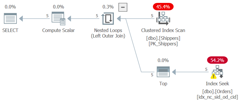 Figure 3: Execution plan for Query 3
The plan scans five rows in the clustered index on Shippers. Per shipper, the plan applies a seek against a covering index on Orders, where (shipperid, orderdate) are the index leading keys, going straight to the last row in each shipper section at the leaf level to pull the maximum order date for the current shipper. Since we have only five shippers, there are only five index seek operations, resulting in a very efficient plan. Here are the performance measures that I got when I executed the CTE’s inner query:
duration: 0 ms, CPU: 0 ms, reads: 15
However, when you run the complete solution (we’ll call it Query 4), you get a completely different plan, as shown in Figure 4.
 Figure 4: Execution plan for Query 4
What happened is that SQL Server unnested the table expression, converting the solution to a logical equivalent of a grouped query, resulting in a full scan of the index on Orders. Here are the performance numbers that I got for this solution:
duration: 316 ms, CPU: 281 ms, reads: 3854
What we need here is to prevent the unnesting of the table expression from taking place, so that the inner query would get optimized with seeks against the index on Orders, and for the outer query to just result in an addition of a Filter operator in the plan. You achieve this using our trick by adding a TOP filter to the inner query, like so (we’ll call this solution Query 5):
  WITH C AS
  (
    SELECT TOP (9223372036854775807) S.shipperid,
      (SELECT MAX(O.orderdate)
       FROM dbo.Orders AS O
       WHERE O.shipperid = S.shipperid) AS maxod
    FROM dbo.Shippers AS S
  )
  SELECT shipperid, maxod
  FROM C
  WHERE maxod >= '20180101';
The plan for this solution is shown in Figure 5.
 Figure 5: Execution plan for Query 5
The plan shows that the desired effect was achieved, and accordingly the performance numbers confirm this:
duration: 0 ms, CPU: 0 ms, reads: 15
So, our testing confirms that SQL Server handles substitution/unnesting of CTEs just like it does for derived tables. This means that you shouldn’t prefer one over the other due to optimization reasons, rather due to conceptual differences that matter to you, as discussed in Part 5.
Persistency
A common misconception concerning CTEs and named table expressions in general is that they serve as some sort of a persistency vehicle. Some think that SQL Server persists the result set of the inner query to a work table, and that the outer query actually interacts with that work table. In practice, regular nonrecursive CTEs and derived tables don’t get persisted. I described the unnesting logic that SQL Server applies when optimizing a query involving table expressions, resulting in a plan that interacts straight with the underlying base tables. Note that the optimizer may choose to use work tables to persist intermediate result sets if it makes sense to do so either for performance reasons, or others, such as Halloween protection. When it does so, you see Spool or Index Spool operators in the plan. However, such choices are unrelated to the use of table expressions in the query.
Recursive CTEs
There are a couple of exceptions in which SQL Server does persist the table expression’s data. One is the use of indexed views. If you create a clustered index on a view, SQL Server persists the inner query’s result set in the view’s clustered index, and keeps it in sync with any changes in the underlying base tables. The other exception is when you use recursive queries. SQL Server needs to persist the intermediate result sets of the anchor and recursive queries in a spool so that it can access the last round’s result set represented by the recursive reference to the CTE name every time the recursive member is executed.
To demonstrate this I’ll use one of the recursive queries from Part 6 in the series.
Use the following code to create the Employees table in the tempdb database, populate it with sample data, and create a supporting index:
  SET NOCOUNT ON;

  USE tempdb;

  DROP TABLE IF EXISTS dbo.Employees;
  GO

  CREATE TABLE dbo.Employees
  (
    empid   INT         NOT NULL
    CONSTRAINT PK_Employees PRIMARY KEY,
    mgrid   INT         NULL
    CONSTRAINT FK_Employees_Employees REFERENCES dbo.Employees,
    empname VARCHAR(25) NOT NULL,
    salary  MONEY       NOT NULL,
    CHECK (empid <> mgrid)
  );

  INSERT INTO dbo.Employees(empid, mgrid, empname, salary)
  VALUES(1,  NULL, 'David'  , $10000.00),
        (2,     1, 'Eitan'  ,  $7000.00),
        (3,     1, 'Ina'    ,  $7500.00),
        (4,     2, 'Seraph' ,  $5000.00),
        (5,     2, 'Jiru'   ,  $5500.00),
        (6,     2, 'Steve'  ,  $4500.00),
        (7,     3, 'Aaron'  ,  $5000.00),
        (8,     5, 'Lilach' ,  $3500.00),
        (9,     7, 'Rita'   ,  $3000.00),
        (10,    5, 'Sean'   ,  $3000.00),
        (11,    7, 'Gabriel',  $3000.00),
        (12,    9, 'Emilia' ,  $2000.00),
        (13,    9, 'Michael',  $2000.00),
        (14,    9, 'Didi'   ,  $1500.00);

  CREATE UNIQUE INDEX idx_unc_mgrid_empid
  ON dbo.Employees(mgrid, empid)
  INCLUDE(empname, salary);
  GO
I used the following recursive CTE to return all subordinates of an input subtree root manager, using employee 3 as the input manager in this example:
DECLARE @root AS INT = 3;

  WITH C AS
  (
    SELECT empid, mgrid, empname
    FROM dbo.Employees
    WHERE empid = @root
    UNION ALL
    SELECT S.empid, S.mgrid, S.empname
    FROM C AS M
      INNER JOIN dbo.Employees AS S
      ON S.mgrid = M.empid
  )
  SELECT empid, mgrid, empname
  FROM C;
The plan for this query (we’ll call it Query 6) is shown in Figure 6.
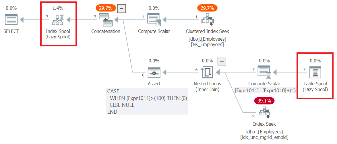 Figure 6: Execution plan for Query 6
Observe that the very first thing that happens in the plan, to the right of the root SELECT node, is the creation of a B-tree-based work table represented by the Index Spool operator. The top part of the plan handles the anchor member’s logic. It pulls the input employee row’s from the clustered index on Employees and writes it to the spool. The bottom part of the plan represents the recursive member’s logic. It is executed repeatedly until it returns an empty result set. The outer input to the Nested Loops operator obtains the managers from the previous round from the spool (Table Spool operator). The inner input uses an Index Seek operator against a nonclustered index created on Employees(mgrid, empid) to obtain the direct subordinates of the managers from the previous round. The result set of each execution of the bottom part of the plan is written to the index spool as well. Notice that all in all, 7 rows were written to the spool. One returned by the anchor member, and 6 more returned by all executions of the recursive member.
As an aside, it’s interesting to notice how the plan handles the default maxrecursion limit, which is 100. Observe that the bottom Compute Scalar operator keeps increasing an internal counter called Expr1011 by 1 with each execution of the recursive member. Then, the Assert operator sets a flag to zero if this counter exceeds 100. If this happens SQL Server stops the execution of the query and generates an error.
When not to persist
Back to nonrecursive CTEs, which normally don’t get persisted, it’s on you to figure out from an optimization perspective when it’s a good thing to use them versus actual persistency tools like temporary tables and table variables instead. I’ll go over a couple of examples to demonstrate when each approach is more optimal.
Let’s start with an example where CTEs do better than temporary tables. That’s often the case when you don’t have multiple evaluations of the same CTE, rather, perhaps just a modular solution where each CTE is evaluated only once. The following code (we’ll call it Query 7) queries the Orders table in the Performance database, which has 1,000,000 rows, to return order years in which more than 70 distinct customers placed orders:
  USE PerformanceV5;

  WITH C1 AS
  (
    SELECT YEAR(orderdate) AS orderyear, custid
    FROM dbo.Orders
  ),
  C2 AS
  (
    SELECT orderyear, COUNT(DISTINCT custid) AS numcusts
    FROM C1
    GROUP BY orderyear
  )
  SELECT orderyear, numcusts
  FROM C2
  WHERE numcusts > 70;
This query generates the following output:
  orderyear   numcusts
  ----------- -----------
  2015        992
  2017        20000
  2018        20000
  2019        20000
  2016        20000
I ran this code using SQL Server 2019 Developer Edition, and got the plan shown in Figure 7.
 Figure 7: Execution plan for Query 7
Notice that the unnesting of the CTE resulted in a plan that pulls the data from an index on the Orders table, and doesn’t involve any spooling of the CTE’s inner query result set. I got the following performance numbers when executing this query on my machine:
duration: 265 ms, CPU: 828 ms, reads: 3970, writes: 0
Now let’s try a solution that uses temporary tables instead of CTEs (we’ll call it Solution 8), like so:
  SELECT YEAR(orderdate) AS orderyear, custid
  INTO #T1
  FROM dbo.Orders;

  SELECT orderyear, COUNT(DISTINCT custid) AS numcusts
  INTO #T2
  FROM #T1
  GROUP BY orderyear;

  SELECT orderyear, numcusts
  FROM #T2
  WHERE numcusts > 70;

  DROP TABLE #T1, #T2;
The plans for this solution are shown in Figure 8.
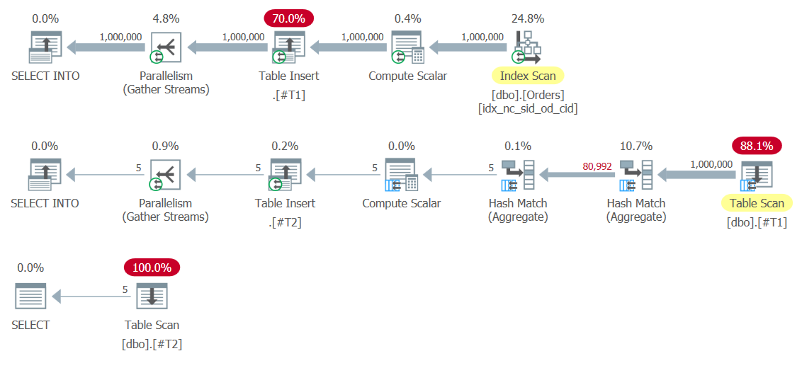 Figure 8: Plans for Solution 8
Notice the Table Insert operators writing the result sets to the temporary tables #T1 and #T2. The first one is especially expensive since it writes 1,000,000 rows to #T1. Here are the performance numbers that I got for this execution:
duration: 454 ms, CPU: 1517 ms, reads: 14359, writes: 359
As you can see, the solution with the CTEs is much more optimal.
When to persist
So is it the case that a modular solution that involves only a single evaluation of each CTE is always preferred to using temporary tables? Not necessarily. In CTE-based solutions that involve many steps, and result in elaborate plans where the optimizer needs to apply lots of cardinality estimates at many different points in the plan, you could end up with accumulated inaccuracies that result in suboptimal choices. One of the techniques to attempt to tackle such cases is to persist some intermediate result sets yourself into temporary tables, and even create indexes on them if needed, giving the optimizer a fresh start with fresh statistics, increasing the likelihood for better quality cardinality estimates that hopefully lead to more optimal choices. Whether this is better than a solution that doesn’t use temporary tables is something that you will need to test. Sometimes the tradeoff of extra cost for persisting intermediate result sets for the sake of getting better quality cardinality estimates will be worth it.
Another typical case where using temporary tables is the preferred approach is when the CTE-based solution has multiple evaluations of the same CTE, and the CTE’s inner query is quite expensive. Consider the following CTE-based solution (we’ll call it Query 9), which matches to each order year and month a different order year and month that has the closest order count:
  WITH OrdCount AS
  (
    SELECT YEAR(orderdate) AS orderyear, MONTH(orderdate) AS ordermonth,
      COUNT(*) AS numorders
    FROM dbo.Orders
    GROUP BY YEAR(orderdate), MONTH(orderdate)
  )
  SELECT O1.orderyear, O1.ordermonth, O1.numorders,
    O2.orderyear AS orderyear2, O2.ordermonth AS ordermonth2,
    O2.numorders AS numorders2
  FROM OrdCount AS O1
  CROSS APPLY ( SELECT TOP (1) O2.orderyear, O2.ordermonth, O2.numorders
                FROM OrdCount AS O2
                WHERE O2.orderyear <> O1.orderyear
                  OR O2.ordermonth <> O1.ordermonth
                ORDER BY ABS(O1.numorders - O2.numorders),
                  O2.orderyear, O2.ordermonth ) AS O2;
This query generates the following output:
  orderyear   ordermonth  numorders   orderyear2  ordermonth2 numorders2
  ----------- ----------- ----------- ----------- ----------- -----------
  2016        1           21262       2017        3           21267
  2019        1           21227       2016        5           21229
  2019        2           19145       2018        2           19125
  2018        4           20561       2016        9           20554
  2018        5           21209       2019        5           21210
  2018        6           20515       2016        11          20513
  2018        7           21194       2018        10          21197
  2017        9           20542       2017        11          20539
  2017        10          21234       2019        3           21235
  2017        11          20539       2019        4           20537
  2017        12          21183       2016        8           21185
  2018        1           21241       2019        7           21238
  2016        2           19844       2019        12          20184
  2018        3           21222       2016        10          21222
  2016        4           20526       2019        9           20527
  2019        4           20537       2017        11          20539
  2017        5           21203       2017        8           21199
  2019        6           20531       2019        9           20527
  2017        7           21217       2016        7           21218
  2018        8           21283       2017        3           21267
  2018        10          21197       2017        8           21199
  2016        11          20513       2018        6           20515
  2019        11          20494       2017        4           20498
  2018        2           19125       2019        2           19145
  2016        3           21211       2016        12          21212
  2019        3           21235       2017        10          21234
  2016        5           21229       2019        1           21227
  2019        5           21210       2016        3           21211
  2017        6           20551       2016        9           20554
  2017        8           21199       2018        10          21197
  2018        9           20487       2019        11          20494
  2016        10          21222       2018        3           21222
  2018        11          20575       2016        6           20571
  2016        12          21212       2016        3           21211
  2019        12          20184       2018        9           20487
  2017        1           21223       2016        10          21222
  2017        2           19174       2019        2           19145
  2017        3           21267       2016        1           21262
  2017        4           20498       2019        11          20494
  2016        6           20571       2018        11          20575
  2016        7           21218       2017        7           21217
  2019        7           21238       2018        1           21241
  2016        8           21185       2017        12          21183
  2019        8           21189       2016        8           21185
  2016        9           20554       2017        6           20551
  2019        9           20527       2016        4           20526
  2019        10          21254       2016        1           21262
  2015        12          1018        2018        2           19125
  2018        12          21225       2017        1           21223

  (49 rows affected)
The plan for Query 9 is shown in Figure 9.
 Figure 9: Execution Plan for Query 9
The top part of the plan corresponds to the instance of the OrdCount CTE that is aliased as O1. This reference results in one evaluation of the CTE OrdCount. This part of the plan pulls the rows from an index on the Orders table, groups them by year and month, and aggregates the count of orders per group, resulting in 49 rows. The bottom part of the plan corresponds to the correlated derived table O2, which is applied per row from O1, hence is executed 49 times. Each execution queries the OrdCount CTE, and therefore results in a separate evaluation of the CTE’s inner query. You can see that the bottom part of the plan scans all rows from the index on Orders, groups and aggregates them. You basically get a total of 50 evaluations of the CTE, resulting in 50 times scanning the 1,000,000 rows from Orders, grouping and aggregating them. It doesn’t sound like a very efficient solution. Here are the performance measures that I got when executing this solution on my machine:
duration: 16 seconds, CPU: 56 seconds, reads: 130404, writes: 0
Given that there are only a few dozen months involved, what would be much more efficient is to use a temporary table to store the result of a single activity that groups and aggregates the rows from Orders, and then have both the outer and inner inputs of the APPLY operator interact with the temporary table. Here’s the solution (we’ll call it Solution 10) using a temporary table instead of the CTE:
  SELECT YEAR(orderdate) AS orderyear, MONTH(orderdate) AS ordermonth,
    COUNT(*) AS numorders
  INTO #OrdCount
  FROM dbo.Orders
  GROUP BY YEAR(orderdate), MONTH(orderdate);

  SELECT O1.orderyear, O1.ordermonth, O1.numorders,
    O2.orderyear AS orderyear2, O2.ordermonth AS ordermonth2,
    O2.numorders AS numorders2
  FROM #OrdCount AS O1
  CROSS APPLY ( SELECT TOP (1) O2.orderyear, O2.ordermonth, O2.numorders
                FROM #OrdCount AS O2
                WHERE O2.orderyear <> O1.orderyear
                  OR O2.ordermonth <> O1.ordermonth
                ORDER BY ABS(O1.numorders - O2.numorders),
                  O2.orderyear, O2.ordermonth ) AS O2;

  DROP TABLE #OrdCount;
Here there’s not much point in indexing the temporary table, since the TOP filter is based on a computation in its ordering specification, and hence a sort is unavoidable. However, it could very well be that in other cases, with other solutions, it would also be relevant for you to consider indexing your temporary tables. At any rate, the plan for this solution is shown in Figure 10.
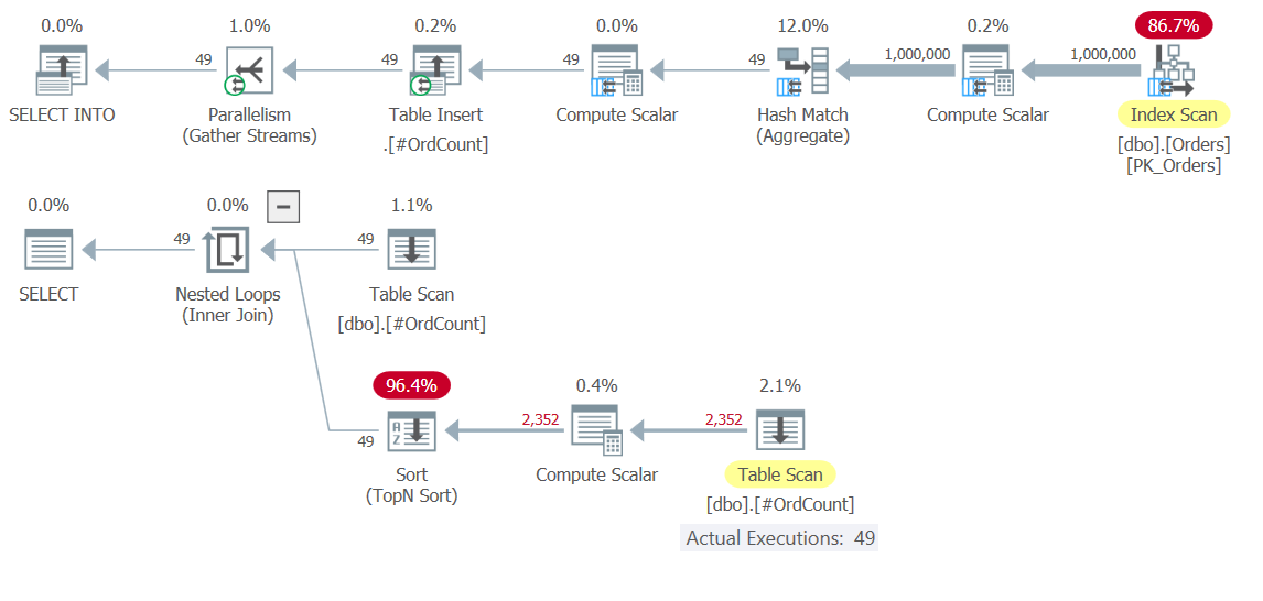 Figure 10: Execution plans for Solution 10
Observe in the top plan how the heavy lifting involving scanning 1,000,000 rows, grouping and aggregating them, happens only once. 49 rows are written to the temporary table #OrdCount, and then the bottom plan interacts with the temporary table for both the outer and inner inputs of the Nested Loops operator, which handles the APPLY operator’s logic.
Here are the performance numbers that I got for the execution of this solution:
duration: 0.392 seconds, CPU: 0.5 seconds, reads: 3636, writes: 3
It’s faster in orders of magnitude than the CTE-based solution.
What’s next?
In this article I started the coverage of optimization considerations related to CTEs. I showed that the unnesting/substitution process that takes place with derived tables works the same way with CTEs. I also discussed the fact that nonrecursive CTEs don’t get persisted and explained that when persistency is an important factor for the performance of your solution, you have to handle it yourself by using tools like temporary tables and table variables. Next month I’ll continue the discussion by covering additional aspects of CTE optimization.


