
DATE_BUCKET and DATETRUNC Improve Optimization of Time-Based Grouping
Time-based grouping and aggregation are common in analyzing data using T-SQL—for example, grouping sales orders by year or by week and computing order counts per group. When you apply time-based grouping, you often group the data by expressions that manipulate date and time columns with functions such as YEAR, MONTH, and DATEPART. Such manipulation typically inhibits the optimizer’s ability to rely on index order. Before SQL Server 2022, there was a workaround that enabled relying on index order, but besides being quite ugly, it had its cost, and the tradeoff wasn’t always acceptable.
SQL Server 2022 introduces new ways to apply time-based grouping using the DATE_BUCKET and DATETRUNC functions. With the DATE_BUCKET function, besides being a flexible tool for handling time-series data, the optimizer can rely on index order when using it for grouping purposes. That’s been the case since the function’s inception in the first public preview of SQL Server 2022 (CTP 2.0). Starting with SQL Server 2022 RC1, that’s also the case with the DATETRUNC function.
I’ll start by presenting the optimization issue found using the older functions, describe the older workaround, and then present the optimization with the newer tools. I’ll also describe cases where you might still need to use the older workaround.
In my examples, I’ll use the sample database TSQLV6. You can download the script file to create and populate this database here and find its ER diagram here.
Important: All testing of examples in this article was done on SQL Server 2022 RC1. Feature availability and optimization could change in future builds of the product.
Optimization of Traditional Time-Based Grouping
Usually, when you group data by unmanipulated columns, SQL Server can apply an order-based group algorithm (Stream Aggregate) that relies on index order. Consider the following query, which I’ll refer to as Query 1, as an example:
USE TSQLV6;

SELECT orderdate, COUNT(*) AS numorders
FROM Sales.Orders
GROUP BY orderdate;
Figure 1 shows the plan for Query 1.
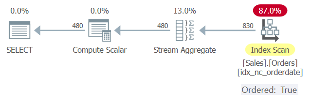 Figure 1: Plan for Query 1
There’s an index called idx_nc_orderdate defined on the Sales.Orders table, with orderdate as the key. This plan scans the index in key order and applies a Stream Aggregate algorithm to the preordered data without requiring explicit sorting.
However, suppose you group the data by expressions that manipulate columns, such as with most date and time-related functions. In that case, this will typically inhibit the optimizer’s ability to rely on index order. The optimizer can still rely on an index for coverage purposes but not on its order.
Consider the following query, which I’ll refer to as Query 2:
SELECT orderyear, COUNT(*) AS numorders
FROM Sales.Orders
CROSS APPLY (VALUES(YEAR(orderdate))) AS D(orderyear)
GROUP BY orderyear;
Theoretically, Microsoft could have added logic to the optimizer to recognize that it could rely on index order here since date order implies year order, but it doesn’t.
Figure 2 shows the plan for Query 2.
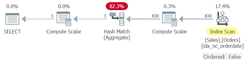 Figure 2: Plan for Query 2
When not finding preordered data, the optimizer can either force explicit sorting in the plan and still use a Stream Aggregate algorithm or a Hash Match (Aggregate) algorithm, which does not have an ordering requirement. In this example, the optimizer opted for the latter.
To verify that the use of a Stream Aggregate algorithm would require explicit sorting, you can force this algorithm with a hint, like so (I’ll call this Query 3):
SELECT orderyear, COUNT(*) AS numorders
FROM Sales.Orders
CROSS APPLY (VALUES(YEAR(orderdate))) AS D(orderyear)
GROUP BY orderyear
OPTION(ORDER GROUP);
Or you can encourage the optimizer to use a Stream Aggregate algorithm by adding a presentation ORDER BY list that is aligned with the grouping set, like so (I’ll call this Query 4):
SELECT orderyear, COUNT(*) AS numorders
FROM Sales.Orders
CROSS APPLY (VALUES(YEAR(orderdate))) AS D(orderyear)
GROUP BY orderyear
ORDER BY orderyear;
Query 3 and Query 4 get similar plans with a Stream Aggregate operator that is preceded by a Sort operator, as shown in Figure 3.
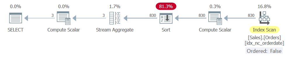 Figure 3: Plan for Query 3 and Query 4
If you’re interested in the details of the costing and scaling of the different grouping algorithms, see the following series:
- Optimization Thresholds – Grouping and Aggregating Data, Part 1
- Optimization Thresholds – Grouping and Aggregating Data, Part 2
- Optimization Thresholds – Grouping and Aggregating Data, Part 3
- Optimization Thresholds – Grouping and Aggregating Data, Part 4
- Optimization Thresholds – Grouping and Aggregating Data, Part 5
The point is that currently, the optimizer is not encoded with the logic to recognize cases where column order implies manipulated column order, and hence the potential to rely on index order, at least with the traditional grouping expressions.
The same applies to the following query, which groups the orders by year and month (I’ll call this Query 5):
SELECT orderyear, ordermonth, COUNT(*) AS numorders
FROM Sales.Orders
CROSS APPLY (VALUES(YEAR(orderdate), MONTH(orderdate)))
               AS D(orderyear, ordermonth)
GROUP BY orderyear, ordermonth;
And the same applies to the following query, which groups the orders by week, assuming Sunday as the first day of the week (I’ll call this Query 6):
SELECT startofweek, COUNT(*) AS numorders
FROM Sales.Orders
CROSS APPLY (VALUES(DATEADD(week,
                      DATEDIFF(week, CAST('19000107' AS DATE), orderdate),
                      CAST('19000107' AS DATE)))) AS D(startofweek)
GROUP BY startofweek;
The Old and Ugly Workaround
Before SQL Server 2022, there was no way I could produce a workaround for the above queries that would rely on the order of the original index on orderdate. However, there was a workaround involving the creation of new indexed computed columns, which the optimizer could then rely upon. The workaround involves the following steps:
- Create computed columns based on the grouping set expressions
- Create an index with the computed columns forming the key
Here’s the code implementing this workaround to support Query 2, as an example:
ALTER TABLE Sales.Orders
ADD corderyear AS YEAR(orderdate);

CREATE NONCLUSTERED INDEX idx_nc_corderyear ON Sales.Orders(corderyear);
Here’s Query 2 again:
SELECT orderyear, COUNT(*) AS numorders
FROM Sales.Orders
CROSS APPLY (VALUES(YEAR(orderdate))) AS D(orderyear)
GROUP BY orderyear;
The new plan for Query 2 is shown in Figure 4.
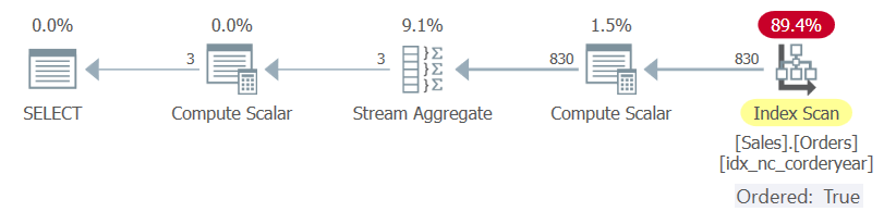 Figure 4: Plan for Query 2 with Old Workaround
The advantage of this workaround is that no code changes are needed for your original query. Notice that even though you could, you didn’t have to change the query to refer to the computed column name corderyear in order to benefit from the new index. The optimizer applied expression matching and realized that the index on the computed column corderyear is based on the same expression as the grouping expression YEAR(orderdate).
The downside of this workaround is that it requires a DDL change to the table, and the addition of a new index. You don’t always have these options available; if you do, there’s extra space needed for the new index and extra modification overhead.
Run the following code to clean up the new index and computed column:
DROP INDEX idx_nc_corderyear ON Sales.Orders;

ALTER TABLE Sales.Orders DROP COLUMN corderyear;
The New and Elegant Workaround Using the DATE_BUCKET Function
As part of a set of new T-SQL features to support time-series scenarios, SQL Server 2022 introduces support for the DATE_BUCKET function. You can find details about this function in my article Bucketizing date and time data, as well as in Aaron Bertrand’s article My Favorite T-SQL Enhancements in SQL Server 2022.
In brief, the DATE_BUCKET function has the following syntax:
DATE_BUCKET( part, width, datetimevalue[, origin] )
The function returns a date and time value of the type of the input date and time value, representing the beginning of the date and time bucket that the input value belongs. Using the first two parameters of the function you define the bucket size, e.g., year, 1. You can explicitly define the starting point for the buckets on the time line using the fourth parameter origin or rely on January 1st, 1900, midnight, as the default.
As an example, consider the following expression:
SELECT DATE_BUCKET( year, 1, CAST('20220718' AS DATE) ) AS startofyear;
This expression assumes bucket arrangement starting with the default origin January 1st, 1900, with a bucket size of one year. It effectively computes the beginning of year date with respect to the input date value, July 18th, 2022. This expression produces the following output:
startofyear
-----------
2022-01-01
The original motivation for adding this function was to support time-series scenarios, where you often need to group data from edge devices such as sensors by date and time buckets, e.g., 15-minute buckets, and apply aggregates per bucket. The pleasant surprise about this function beyond its flexibility is how it gets optimized. Unlike the more traditional date and time functions, which, at least at the time of writing, typically inhibit the optimizer’s ability to rely on index order, Microsoft did encode logic in the optimizer to enable the DATE_BUCKET function to rely on index order.
So, instead of the original Query 2:
SELECT orderyear, COUNT(*) AS numorders
FROM Sales.Orders
CROSS APPLY (VALUES(YEAR(orderdate))) AS D(orderyear)
GROUP BY orderyear;
You can use the DATE_BUCKET function, like so (I’ll refer to this Query 2b):
SELECT YEAR(yearbucket) AS orderyear, COUNT(*) AS numorders
FROM Sales.Orders
CROSS APPLY (VALUES(DATE_BUCKET(year, 1, orderdate))) AS D(yearbucket)
GROUP BY yearbucket;
The plan for Query 2b is shown in Figure 5.
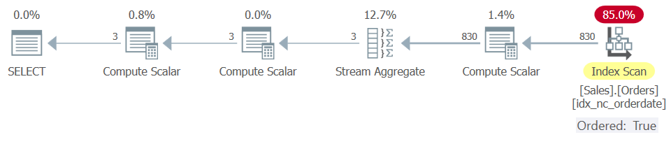 Figure 5: Plan for Query 2b with New Workaround
Similarly, instead of the original Query 5:
SELECT orderyear, ordermonth, COUNT(*) AS numorders
FROM Sales.Orders
CROSS APPLY (VALUES(YEAR(orderdate), MONTH(orderdate)))
               AS D(orderyear, ordermonth)
GROUP BY orderyear, ordermonth;
Use the following (I’ll call this Query 5b):
SELECT
YEAR(yearmonthbucket) AS orderyear,
MONTH(yearmonthbucket) AS ordermonth,
COUNT(*) AS numorders
FROM Sales.Orders
CROSS APPLY (VALUES(DATE_BUCKET(month, 1, orderdate))) AS D(yearmonthbucket)
GROUP BY yearmonthbucket;
Instead of the original Query 6:
SELECT startofweek, COUNT(*) AS numorders
FROM Sales.Orders
CROSS APPLY (VALUES(DATEADD(week,
                      DATEDIFF(week, CAST('19000107' AS DATE), orderdate),
                      CAST('19000107' AS DATE)))) AS D(startofweek)
GROUP BY startofweek;
Use the following (I’ll call this Query 6b):
SELECT startofweek, COUNT(*) AS numorders
FROM Sales.Orders
CROSS APPLY (VALUES(DATE_BUCKET(week, 1, orderdate, CAST('19000107' AS DATE))))
               AS D(startofweek)
GROUP BY startofweek;
Whereas Query 2, Query 5 and Query 6 got plans that could not rely on index order, Query 2b, Query 5b and Query 6b got plans that did.
You get the general idea!
What about the new DATETRUNC function?
SQL Server 2022 also introduces support for the DATETRUNC function. This function has the following syntax:
DATETRUNC( part, datetimevalue )
The function returns a date and time value representing the input value truncated, or floored, to the beginning of the specified part. For instance, if you specify year as the part, you get the input value floored to the beginning of the year. If you specify month as the part, you get the input value floored to the beginning of the month. If the input value’s type is a date and time type, you get an output of the same type and precision. If the input is of a character string type, it is converted to DATETIME2(7), which is also the output type.
For most parts, you could think of the DATETRUNC function as a simplified version of the DATE_BUCKET function, with the same part, width of 1, and no explicit origin.
As an example, consider the following expression:
SELECT DATETRUNC( year, CAST('20220718' AS DATE) ) AS startofyear;
It is equivalent to:
SELECT DATE_BUCKET( year, 1, CAST('20220718' AS DATE) ) AS startofyear;
Both expressions produce the following output:
startofyear
-----------
2022-01-01
Similar to the rewrites you made to queries that use traditional date and time functions to use DATE_BUCKET instead, you could rewrite them to use DATETRUNC instead.
So, instead of the original Query 2:
SELECT orderyear, COUNT(*) AS numorders
FROM Sales.Orders
CROSS APPLY (VALUES(YEAR(orderdate))) AS D(orderyear)
GROUP BY orderyear;
You could use the DATETRUNC function, like so (I’ll refer to this Query 2c):
SELECT YEAR(startofyear) AS orderyear, COUNT(*) AS numorders
FROM Sales.Orders
CROSS APPLY (VALUES(DATETRUNC(year, orderdate))) AS D(startofyear)
GROUP BY startofyear;
Similarly, instead of the original Query 5:
SELECT orderyear, ordermonth, COUNT(*) AS numorders
FROM Sales.Orders
CROSS APPLY (VALUES(YEAR(orderdate), MONTH(orderdate)))
               AS D(orderyear, ordermonth)
GROUP BY orderyear, ordermonth;
You could use the following (I’ll call this Query 5c):
SELECT
YEAR(startofmonth) AS orderyear,
MONTH(startofmonth) AS ordermonth,
COUNT(*) AS numorders
FROM Sales.Orders
CROSS APPLY (VALUES(DATETRUNC(month, orderdate))) AS D(startofmonth)
GROUP BY startofmonth;
Instead of the original Query 6:
SELECT startofweek, COUNT(*) AS numorders
FROM Sales.Orders
CROSS APPLY (VALUES(DATEADD(week,
                      DATEDIFF(week, CAST('19000107' AS DATE), orderdate),
                      CAST('19000107' AS DATE)))) AS D(startofweek)
GROUP BY startofweek;
You could use the following (I’ll call this Query 6c):
SET DATEFIRST 7;

SELECT startofweek, COUNT(*) AS numorders
FROM Sales.Orders
CROSS APPLY (VALUES(DATETRUNC(week, orderdate))) AS D(startofweek)
GROUP BY startofweek;
Although not the case in earlier builds, starting with SQL Server 2022 RC1, the DATETRUNC function can rely on index order for grouping purposes similar to the DATE_BUCKET function. The plans generated for Query 2c, Query 5c, and Query 6c are similar to the ones generated for Query 2b, Query 5b, and Query 6b, respectively. All end up with an ordered index scan and no explicit sorting prior to a Stream Aggregate operator.
What about other manipulations?
Basic grouping is only one example where there’s potential for the optimizer to rely on index order even when manipulating the underlying columns, but where currently, it doesn’t. There are many other examples like filtering, more sophisticated hierarchical grouping with grouping sets, distinctness, joining, and others. For now, you can resolve only some of the cases by revising the code to use the DATE_BUCKET function. For some of the rest of the cases, you can still use the hack with the indexed computed columns if that’s an option and the tradeoff is acceptable. I’ll demonstrate this with filtering and hierarchical time-based grouping with grouping sets.
As an example for filtering, consider classic queries where you need to filter a consecutive period of time like a whole year or a whole month. The recommended way to go is to use a SARGable predicate without manipulating the filtered column. For example, to filter orders placed in 2021, the recommended way to write the query is like so (I’ll call this Query 7):
SELECT orderid, orderdate
FROM Sales.Orders
WHERE orderdate >= '20210101' AND orderdate < '20220101';
The plan for Query 7 is shown in Figure 6.
 Figure 6: Plan for Query 7
As you can see, the plan relies on index order by applying a seek.
You often see people writing queries that filter consecutive time periods by applying functions to the filtered columns, not realizing the optimization implications. For example, using the YEAR function to filter a whole year, like so (I’ll call this Query 8):
SELECT orderid, orderdate
FROM Sales.Orders
WHERE YEAR(orderdate) = 2021;
The plan for this query, which is shown in Figure 7, shows a full scan of the index on orderdate.
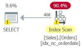 Figure 7: Plan for Query 8
If you’re curious about how filtering with the DATE_BUCKET function is optimized; unlike with grouping, when using this function in a filter predicate, this also inhibits relying on index order. Consider the following query:
SELECT orderid, orderdate
FROM Sales.Orders
WHERE DATE_BUCKET(year, 1, orderdate) = '20210101';
SQL Server’s optimizer doesn’t consider this to be a SARGable predicate, resulting in a plan that scans the index on orderdate, similar to the plan shown in Figure 7.
I’m afraid that the same applies when using the DATETRUNC function:
SELECT orderid, orderdate
FROM Sales.Orders
WHERE DATETRUNC(year, orderdate) = '20210101';
Also here, SQL Server’s optimizer doesn’t consider this to be a SARGable predicate, resulting in a plan that scans the index on orderdate, similar to the plan shown in Figure 7.
Again, potentially the optimization of the new functions could be enhanced in the future to recognize such cases as SARGable and enable a seek in a supporting index, but at the time of writing they are not.
Naturally, the best thing you can do as a developer is to be familiar with best practices and ensure that you write your queries with SARGable predicates, such as Query 6. The problem is that sometimes you have no control over the way the code is written, and you don’t have the option to revise it. In such cases, it’s good to have the option with the indexed computed columns assuming the tradeoff is acceptable. For instance, suppose the original code in the application is Query 7, and you don’t have the option to revise it to Query 6. You could create the following computed column and supporting covering index:
ALTER TABLE Sales.Orders
ADD corderyear AS YEAR(orderdate);

CREATE NONCLUSTERED INDEX idx_nc_corderyear_i_od_oid ON Sales.Orders(corderyear)
INCLUDE(orderdate, orderid);
Rerun Query 7:
SELECT orderid, orderdate
FROM Sales.Orders
WHERE YEAR(orderdate) = 2021;
The plan for Query 7, which is shown in Figure 8, applies a seek against the new index.
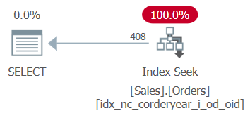 Figure 8: New plan for Query 7
Run the following code for cleanup:
DROP INDEX idx_nc_corderyear_i_od_oid ON Sales.Orders;

ALTER TABLE Sales.Orders DROP COLUMN corderyear;
The same trick can also be applied in hierarchical time-based grouping with grouping sets, such as when using the ROLLUP option. Consider the following query as an example (I’ll call it Query 9):
SELECT orderyear, ordermonth, orderday, COUNT(*) AS numorders
FROM Sales.Orders
CROSS APPLY (VALUES(YEAR(orderdate), MONTH(orderdate), DAY(orderdate)))
               AS D(orderyear, ordermonth, orderday)
GROUP BY ROLLUP(orderyear, ordermonth, orderday);
The plan for Query 9 is shown in Figure 9.
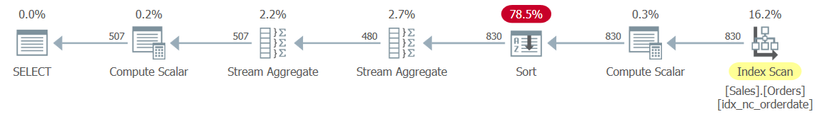 Figure 9: Plan for Query 9
The plan scans the input data only once, but then it sorts it. The first Stream Aggregate operator handles the base grouping, and the second handles the rolling up of the aggregates based on the time hierarchy. Theoretically, SQL Server’s optimizer could rely on the order of the index on orderdate and avoid a sort here. However, similar to the earlier examples of grouped queries, it doesn’t, resulting in explicit sorting in the plan.
An attempt to replace the expressions using the YEAR, MONTH and DAY functions with ones using the DATE_BUCKET function, at least in a trivial way, doesn’t help here. You still get a sort in the plan. What would prevent a sort is to emulate the use of the ROLLUP option by writing multiple grouped queries for the different grouping sets, some using the DATE_BUCKET function, and unifying the results, like so (I’ll call this Query 10):
SELECT
YEAR(orderdate) AS orderyear,
MONTH(orderdate) AS ordermonth,
DAY(orderdate) AS orderday,
COUNT(*) AS numorders
FROM Sales.Orders
GROUP BY orderdate

UNION ALL

SELECT
YEAR(yearmonthbucket) AS orderyear,
MONTH(yearmonthbucket) AS ordermonth,
NULL AS orderday,
COUNT(*) AS numorders
FROM Sales.Orders
CROSS APPLY (VALUES(DATE_BUCKET(month, 1, orderdate))) AS D(yearmonthbucket)
GROUP BY yearmonthbucket

UNION ALL

SELECT
YEAR(yearbucket) AS orderyear,
NULL AS ordermonth,
NULL AS orderday,
COUNT(*) AS numorders
FROM Sales.Orders
CROSS APPLY (VALUES(DATE_BUCKET(year, 1, orderdate))) AS D(yearbucket)
GROUP BY yearbucket

UNION ALL

SELECT
NULL AS orderyear,
NULL AS ordermonth,
NULL AS orderday,
COUNT(*) AS numorders
FROM Sales.Orders
GROUP BY GROUPING SETS(());
The plan for this query is shown in Figure 10.
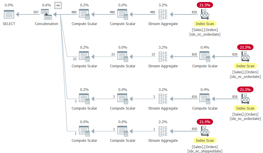 Figure 10: Plan for Query 10
Indeed there’s no sorting in the plan, and this plan has linear scaling compared to N Log N scaling when sorting is involved; however, there are four scans of the input data instead of one. So, which plan is better depends on the input size. You also need to consider the loss of programmatic benefits due to the much more verbose coding here.
If it’s important for you to keep Query 9 as your solution, plus avoid the sort in the plan, and you’re willing to accept the tradeoff involved with adding computed columns and indexing them, the old trick works here. Here’s the code to add the computed columns and the indexes:
ALTER TABLE Sales.Orders
ADD corderyear AS YEAR(orderdate),
    cordermonth AS MONTH(orderdate),
    corderday AS DAY(orderdate);

CREATE NONCLUSTERED INDEX idx_nc_corderymd ON Sales.Orders(corderyear, cordermonth, corderday);
Rerun Query 9:
SELECT orderyear, ordermonth, orderday, COUNT(*) AS numorders
FROM Sales.Orders
CROSS APPLY (VALUES(YEAR(orderdate), MONTH(orderdate), DAY(orderdate)))
               AS D(orderyear, ordermonth, orderday)
GROUP BY ROLLUP(orderyear, ordermonth, orderday);
Now you get the plan shown in Figure 11, with only one scan of the input and no explicit sorting.
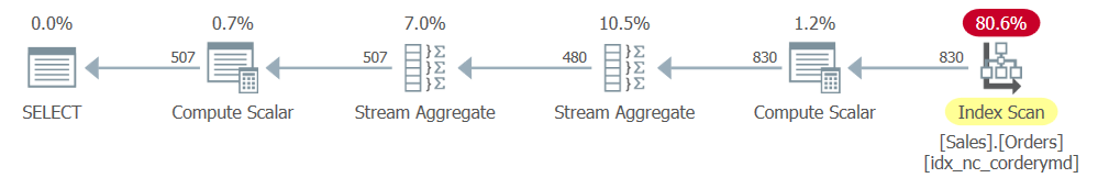 Figure 11: New Plan for Query 9
It’s good to know that the old trick works here, but naturally, it would have been better if the optimizer recognized that it could rely on the index on the orderdate column to begin with.
Run the following code for cleanup:
DROP INDEX idx_nc_corderymd ON Sales.Orders;

ALTER TABLE Sales.Orders DROP COLUMN corderyear, cordermonth, corderday;
Conclusion
In this article I showed that when grouping data by expressions that manipulate date and time columns with traditional functions like DATEPART, YEAR, MONTH and DAY, such manipulation typically inhibits the optimizer’s ability to rely on index order even when theoretically it could have been beneficial. It’s great to see that with the new DATE_BUCKET and DATETRUNC functions in SQL Server 2022, Microsoft did add logic to the optimizer to enable relying on index order. Consequently, for now, you’d be better off in some cases revising grouped queries that use traditional functions to use DATE_BUCKET or DATETRUNC instead. The tradeoff is that the code will be a bit less natural than it was originally.
Ideally, in the future, Microsoft will add logic to the optimizer so that it can rely on index order also when manipulating the underlying columns with traditional date and time functions. The same goes for handling filtering tasks, more sophisticated grouping, and any situation where potentially index ordering could be relevant. This will enable each role in the data platform ecosystem to focus on what they’re supposed to. It will enable developers to write solutions that are more natural by avoiding query rewrites just for the sake of performance. It will enable DBAs to apply more natural tuning by creating indexes only on the original date and time columns and avoiding the need to use costly hacks like indexed computed columns.
At any rate, the addition of the DATE_BUCKET and DATETRUNC functions to T-SQL and their optimization is fantastic, and we can only hope to see many more great additions to T-SQL like this one in the future.
