Optimization Thresholds – Grouping and Aggregating Data, Part 2

This article is the second in a series about optimization thresholds related to grouping and aggregating data. In Part 1, I provided the reverse-engineered formula for the Stream Aggregate operator cost. I explained that this operator needs to consume the rows ordered by the grouping set (any order of its members), and that when the data is obtained preordered from an index, you get linear scaling with respect to the number of rows and the number of groups. Also, there’s no memory grant needed in such a case.

In this article, I focus on the costing and scaling of a stream aggregate-based operation when the data isn’t obtained preordered from an index, rather, has to be sorted first.

In my examples, I’ll use the PerformanceV3 sample database, like in Part 1. You can download the script that creates and populates this database from here. Before you run the examples from this article, make sure that you run the following code first to drop a couple of unneeded indexes:

DROP INDEX idx_nc_sid_od_cid ON dbo.Orders;
DROP INDEX idx_unc_od_oid_i_cid_eid ON dbo.Orders;

The only two indexes that should be left on this table are idx_cl_od (clustered with orderdate as the key) and PK_Orders (nonclustered with orderid as the key).

Sort + Stream Aggregate

The focus of this article is to try and figure out how a stream aggregate operation scales when the data is not preordered by the grouping set. Since the Stream Aggregate operator has to process the rows ordered, if they are not preordered in an index, the plan has to include an explicit Sort operator. So the cost of the aggregate operation you should take into account is the sum of the costs of the Sort + Stream Aggregate operators.

I’ll use the following query (we’ll call it Query 1) to demonstrate a plan involving such optimization:

SELECT shipperid, MAX(orderdate) AS maxod
  FROM (SELECT TOP (100) * FROM dbo.Orders) AS D
  GROUP BY shipperid;

The plan for this query is shown in Figure 1.

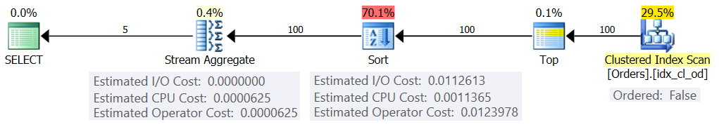
Figure 1: Plan for Query 1

The reason I use a table expression with a TOP filter is to control the exact number of (estimated) rows involved in the grouping and aggregation. Applying controlled changes makes it easier to try and reverse-engineer the costing formulas.

If you’re wondering why filter such a small number of rows in this example, it has to do with the optimization thresholds that make this strategy preferred to the Hash Aggregate algorithm. In Part 3 I’ll describe the costing and scaling of the hash alternative. In cases where the optimizer doesn’t choose a stream aggregate operation by itself, e.g., when large numbers of rows are involved, you can always force it with the hint OPTION(ORDER GROUP) during the research process. When focusing on the costing of serial plans, you can obviously add a MAXDOP 1 hint to eliminate parallelism.

As mentioned, to evaluate the cost and scaling of a nonpreordered stream aggregate algorithm, you need to take into account the sum of the Sort + Stream Aggregate operators. You already know the costing formula for the Stream Aggregate operator from Part 1:

In our query we have 100 estimated input rows and 5 estimated output groups (5 distinct shipper IDs estimated based on density information). So the cost of the Stream Aggregate operator in our plan is:

Let's try and figure out the costing formula for the Sort operator. Remember, our focus is the estimated cost and scaling because our ultimate goal is to figure out optimization thresholds where the optimizer changes its choices from one strategy to another.

The I/O cost estimate seems to be fixed: 0.0112613. I get the same I/O cost irrespective of factors like number of rows, number of sort columns, data type, and so on. This is probably to account for some anticipated I/O work.

As for the CPU cost, alas, Microsoft doesn’t publicly expose the exact algorithms that they use for sorting. However, among the common algorithms used for sorting by database engines in general are different implementations of merge sort and quicksort. Thanks to efforts made by Paul White, who’s fond of looking at Windows debugger stack traces (not all of us have the stomach for this), we have a bit more insight into the topic, published in his series “Internals of the Seven SQL Server Sorts.” According to Paul’s findings, the general sort class (used in the above plan) uses merge sort (first internal, then transitioning to external). In average, this algorithm requires n log n comparisons to sort n items. With this in mind, it’s probably a safe bet as a starting point to assume that the CPU part of the operator’s cost is based on a formula such as:

Of course, this could be an oversimplification of the actual costing formula that Microsoft uses, but absent any documentation on the matter, this is an initial best guess.

Next, you can obtain the sort CPU costs from two query plans produced for sorting different numbers of rows, say 1000 and 2000, and based on those and the above formula, reverse engineer the comparison cost and startup cost. For this purpose, you don’t have to use a grouped query; it’s enough to just do a basic ORDER BY. I’ll use the following two queries (we’ll call them Query 2 and Query 3):

SELECT orderid % 1000000000 as myorderid
  FROM (SELECT TOP (1000) * FROM dbo.Orders) AS D
  ORDER BY myorderid;

  SELECT orderid % 1000000000 as myorderid
  FROM (SELECT TOP (2000) * FROM dbo.Orders) AS D
  ORDER BY myorderid;

The point in ordering by the result of a computation is to force a Sort operator to be used in the plan.

Figure 2 shows the relevant parts of the two plans:

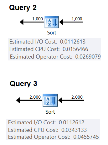
Figure 2: Plans for Query 2 and Query 3

To try and infer the cost of one comparison, you would use the following formula:

As for the startup cost, you can infer it based on either plan, e.g., based on the plan that sorts 2000 rows:

And thus our Sort CPU cost formula becomes:

Using similar techniques, you will find that factors like the average row size, number of ordering columns and their data types do not affect the estimated sort CPU cost. The only factor that seems to be relevant is the estimated number of rows. Note that the sort will need a memory grant, and the grant is proportional to the number of rows (not groups) and the average row size. But our focus currently is the estimated operator cost, and it appears that this estimate is affected only by the estimated number of rows.

This formula seems to predict the CPU cost well up to a threshold of about 5,000 rows. Try it with the following numbers: 100, 200, 300, 400, 500, 1000, 2000, 3000, 4000, 5000:

SELECT
    numrows,
    9.99127891201865E-05 + numrows * LOG(numrows) * 2.25061348918698E-06 AS predicatedcost
  FROM (VALUES(100), (200), (300), (400), (500), (1000), (2000), (3000), (4000), (5000))
    AS D(numrows);

Compare what the formula predicts and the estimated CPU costs that the plans show for the following queries:

SELECT orderid % 1000000000 as myorderid
  FROM (SELECT TOP (100) * FROM dbo.Orders) AS D
  ORDER BY myorderid;

  SELECT orderid % 1000000000 as myorderid
  FROM (SELECT TOP (200) * FROM dbo.Orders) AS D
  ORDER BY myorderid;

  SELECT orderid % 1000000000 as myorderid
  FROM (SELECT TOP (300) * FROM dbo.Orders) AS D
  ORDER BY myorderid;

  SELECT orderid % 1000000000 as myorderid
  FROM (SELECT TOP (400) * FROM dbo.Orders) AS D
  ORDER BY myorderid;

  SELECT orderid % 1000000000 as myorderid
  FROM (SELECT TOP (500) * FROM dbo.Orders) AS D
  ORDER BY myorderid;

  SELECT orderid % 1000000000 as myorderid
  FROM (SELECT TOP (1000) * FROM dbo.Orders) AS D
  ORDER BY myorderid;

  SELECT orderid % 1000000000 as myorderid
  FROM (SELECT TOP (2000) * FROM dbo.Orders) AS D
  ORDER BY myorderid;

  SELECT orderid % 1000000000 as myorderid
  FROM (SELECT TOP (3000) * FROM dbo.Orders) AS D
  ORDER BY myorderid;

  SELECT orderid % 1000000000 as myorderid
  FROM (SELECT TOP (4000) * FROM dbo.Orders) AS D
  ORDER BY myorderid;

  SELECT orderid % 1000000000 as myorderid
  FROM (SELECT TOP (5000) * FROM dbo.Orders) AS D
  ORDER BY myorderid;

I got the following results:

  numrows     predicatedcost  estimatedcost  ratio
  ----------- --------------- -------------- -------
   100        0.0011363       0.0011365      1.00018
   200        0.0024848       0.0024849      1.00004
   300        0.0039510       0.0039511      1.00003
   400        0.0054937       0.0054938      1.00002
   500        0.0070933       0.0070933      1.00000
  1000        0.0156466       0.0156466      1.00000
  2000        0.0343133       0.0343133      1.00000
  3000        0.0541576       0.0541576      1.00000
  4000        0.0747667       0.0747665      1.00000
  5000        0.0959445       0.0959442      1.00000

The column predictedcost shows the predication based on our reverse-engineered formula, the column estimatedcost shows the estimated cost that appears in the plan, and the column ratio shows the ratio between the latter and the former.

The predication seems pretty accurate up to 5,000 rows. However, with numbers greater than 5,000, our reverse-engineered formula stops working well. The following query gives you the predications for 6K, 7K, 10K, 20K, 100K and 200K rows:

SELECT
    numrows,
    9.99127891201865E-05 + numrows * LOG(numrows) * 2.25061348918698E-06 AS predicatedcost
  FROM (VALUES(6000), (7000), (10000), (20000), (100000), (200000)) AS D(numrows);

Use the following queries to get the estimated CPU costs from the plans (note the hint to force a serial plan since with larger numbers of rows it’s more likely that you will get a parallel plan where the costing formulas are adjusted for parallelism):

SELECT orderid % 1000000000 as myorderid
  FROM (SELECT TOP (6000) * FROM dbo.Orders) AS D
  ORDER BY myorderid
  OPTION(MAXDOP 1);

  SELECT orderid % 1000000000 as myorderid
  FROM (SELECT TOP (7000) * FROM dbo.Orders) AS D
  ORDER BY myorderid
  OPTION(MAXDOP 1);

  SELECT orderid % 1000000000 as myorderid
  FROM (SELECT TOP (10000) * FROM dbo.Orders) AS D
  ORDER BY myorderid
  OPTION(MAXDOP 1);

  SELECT orderid % 1000000000 as myorderid
  FROM (SELECT TOP (20000) * FROM dbo.Orders) AS D
  ORDER BY myorderid
  OPTION(MAXDOP 1);

  SELECT orderid % 1000000000 as myorderid
  FROM (SELECT TOP (100000) * FROM dbo.Orders) AS D
  ORDER BY myorderid
  OPTION(MAXDOP 1);

  SELECT orderid % 1000000000 as myorderid
  FROM (SELECT TOP (200000) * FROM dbo.Orders) AS D
  ORDER BY myorderid
  OPTION(MAXDOP 1);

I got the following results:

  numrows     predicatedcost  estimatedcost  ratio
  ----------- --------------- -------------- ------
       6000   0.117575        0.160970       1.3691
       7000   0.139583        0.244848       1.7541
      10000   0.207389        0.603420       2.9096
      20000   0.445878        1.311710       2.9419
     100000   2.591210        7.623920       2.9422
     200000   5.494330       16.165700       2.9423

As you can see, beyond 5,000 rows our formula becomes less and less accurate, but curiously, the accuracy ratio stabilizes on about 2.94 at around 20,000 rows. This implies that with large numbers our formula still applies, only with a higher comparison cost, and that roughly between 5,000 and 20,000 rows, it transitions gradually from the lower comparison cost to the higher one. But what could explain the difference between the small scale and the large scale? The good news is that the answer is not as complex as reconciling quantum mechanics and general relativity with string theory. It’s just that at the smaller scale Microsoft wanted to account for the fact that the CPU cache is likely to be used, and for costing purposes, they assume a fixed cache size.

So, to figure out the comparison cost at the large scale, you want to use the sort CPU costs from two plans for numbers above 20,000. I’ll use 100,000 and 200,000 rows (last two rows in table above). Here’s the formula to infer the comparison cost:

Next, here’s the formula to infer the startup cost based on the plan for 200,000 rows:

It could very well be that the startup cost for the small and large scales is the same, and that the difference we got is due to rounding errors. At any rate, with large numbers of rows, the startup cost becomes negligible compared to the comparisons’ cost.

In summary, here’s the formula for the Sort operator’s CPU cost for large numbers (>= 20000):

Let’s test the accuracy of the formula with 500K, 1M and 10M rows. The following code gives you our formula’s predications:

SELECT
    numrows,
    1.35166186417734E-04 + numrows * LOG(numrows) * 6.62193536908588E-06 AS predicatedcost
  FROM (VALUES(500000), (1000000), (10000000)) AS D(numrows);

Use the following queries to get the estimated CPU costs:

SELECT orderid % 1000000000 as myorderid
  FROM (SELECT TOP (500000) * FROM dbo.Orders) AS D
  ORDER BY myorderid
  OPTION(MAXDOP 1);

  SELECT orderid % 1000000000 as myorderid
  FROM (SELECT TOP (1000000) * FROM dbo.Orders) AS D
  ORDER BY myorderid
  OPTION(MAXDOP 1);

  SELECT CHECKSUM(NEWID()) as myorderid
  FROM (SELECT TOP (10000000) O1.orderid
  FROM dbo.Orders AS O1 CROSS JOIN dbo.Orders AS O2) AS D
  ORDER BY myorderid
  OPTION(MAXDOP 1);

I got the following results:

  numrows     predicatedcost  estimatedcost  ratio
  ----------- --------------- -------------- ------
       500000         43.4479        43.448  1.0000
      1000000         91.4856        91.486  1.0000
     10000000       1067.3300      1067.340  1.0000

Looks like our formula for large numbers does pretty well.

Putting it all together

The total cost of applying a stream aggregate with explicit sorting for small numbers of rows (<= 5,000 rows) is:

Figure 3 has an area chart showing how this cost scales.

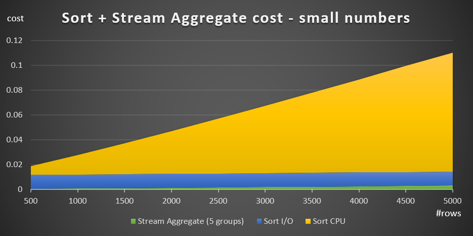
Figure 3: Cost of Sort + Stream Aggregate for small numbers of rows

The sort CPU cost is the most substantial part of the total Sort + Stream aggregate cost. Still, with small numbers of rows, the Stream Aggregate cost and the Sort I/O part of the cost are not entirely negligible. In visual terms, you can clearly see all three parts in the chart.

As for large numbers of rows (>= 20,000), the costing formula is:

I did not see much value in pursuing the exact way the comparison cost transitions from the small to the large scale.

Figure 4 has an area chart showing how the cost scales for large numbers.

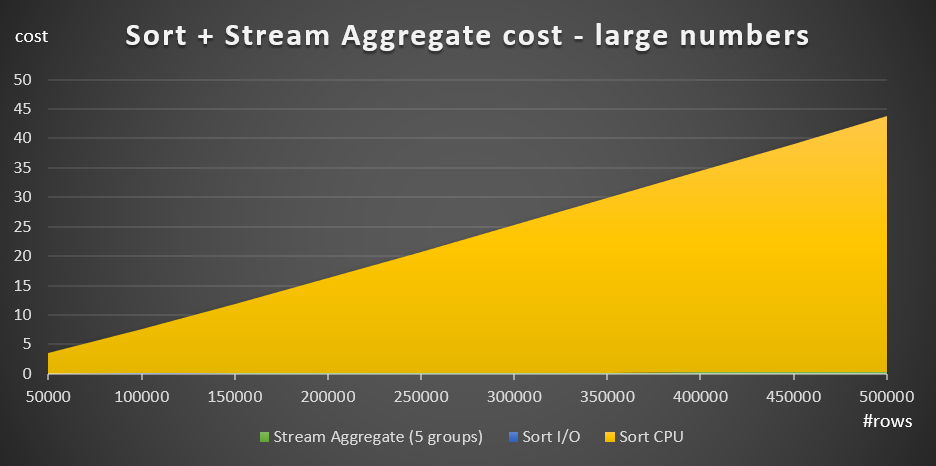
Figure 4: Cost of Sort + Stream Aggregate for large numbers of rows

With large numbers of rows, the Stream Aggregate cost and Sort I/O cost are so negligible compared to the Sort CPU cost that they are not even visible to the naked eye in the chart. In addition, the part of the Sort CPU cost attributed to the startup work is also negligible. Therefore, the only part of the cost calculation that is really meaningful is the total comparison cost:

This means that when you need to evaluate the scaling of the Sort + Stream Aggregate strategy, you can simplify it to this dominant part alone. For instance, if you need to evaluate how the cost would scale from 100,000 rows to 100,000,000 rows, you can use the formula (notice the comparison cost is irrelevant):

This tells you that when the number of rows increases from 100,000 by a factor of 1,000, to 100,000,000, the estimated cost increases by a factor of 1,600.

Scaling from 1,000,000 to 1,000,000,000 rows is computed as:

That is, when the number of rows increases from 1,000,000 by a factor of 1,000, the estimated cost increases by a factor of 1,500.

These are interesting observations about the way the Sort + Stream Aggregate strategy scales. Due to its very low startup cost, and extra linear scaling, you would expect this strategy to do well with very small numbers of rows, but not so well with large numbers. Also, the fact that the Stream Aggregate operator alone represents such a small fraction of the cost compared to when a sort is also needed, tells you that you can get significantly better performance if the situation is such that you are able to create a supporting index.

In the next part of the series, I’ll cover the scaling of the Hash Aggregate algorithm. If you enjoy this exercise of trying to figure out costing formulas, see if you can figure it out for this algorithm. What’s important is to figure out the factors that affect it, the way it scales, and the conditions where it does better than the other algorithms.