
Optimization Thresholds – Grouping and Aggregating Data, Part 3
This article is the third in a series about optimization thresholds for grouping and aggregating data. In Part 1 I covered the preordered Stream Aggregate algorithm. In Part 2 I covered the nonpreordered Sort + Stream Aggregate algorithm. In this part I cover the Hash Match (Aggregate) algorithm, which I’ll refer to simply as Hash Aggregate. I also provide a summary and a comparison between the algorithms I cover in Part 1, Part 2, and Part 3.
I’ll use the same sample database called PerformanceV3, which I used in the previous articles in the series. Just make sure that before you run the examples in the article, you first run the following code to drop a couple of unneeded indexes:
DROP INDEX idx_nc_sid_od_cid ON dbo.Orders;
DROP INDEX idx_unc_od_oid_i_cid_eid ON dbo.Orders;
The only two indexes that should be left on this table are idx_cl_od (clustered with orderdate as the key) and PK_Orders (nonclustered with orderid as the key).
Hash Aggregate
The Hash Aggregate algorithm organizes the groups in a hash table based on some internally chosen hash function. Unlike the Stream Aggregate algorithm, it doesn’t need to consume the rows in group order. Consider the following query (we’ll call it Query 1) as an example (forcing a hash aggregate and a serial plan):
SELECT empid, COUNT(*) AS numorders
  FROM dbo.Orders
  GROUP BY empid
  OPTION (HASH GROUP, MAXDOP 1);
Figure 1 shows the plan for Query 1.
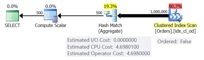
Figure 1: Plan for Query 1
The plan scans the rows from the clustered index using an Ordered: False property (scan isn’t required to deliver the rows ordered by the index key). Typically, the optimizer will prefer to scan the narrowest covering index, which in our case happens to be the clustered index. The plan builds a hash table with the grouped columns and the aggregates. Our query requests an INT-typed COUNT aggregate. The plan actually computes it as a BIGINT-typed value, hence the Compute Scalar operator, applying implicit conversion to INT.
Microsoft doesn’t publicly share the hash algorithms that they use. This is very proprietary technology. Still, in order to illustrate the concept, let’s suppose that SQL Server uses the % 250 (modulo 250) hash function for our query above. Before processing any rows, our hash table has 250 buckets representing the 250 possible outcomes of the hash function (0 through 249). As SQL Server processes each row, it applies the hash function <current empid> % 250. The result is a pointer to one of the buckets in our hash table. If the bucket’s linked list doesn’t yet include the current row’s group, SQL Server adds a new group to the linked list with the group columns (empid in our case) and the initial aggregate value (count 1 in our case). If the group already exists, SQL Server updates the aggregate (adds 1 to the count in our case). For example, suppose that SQL Server happens to process the following 10 rows first:
orderid empid
------- -----
320     3
30      5
660     253
820     3
850     1
1000    255
700     3
1240    253
350     4
400     255
Figure 2 shows three states of the hash table: before any rows are processed, after the first 5 rows are processed, and after the first 10 rows are processed. Each item in the linked list holds the tuple (empid, COUNT(*)).
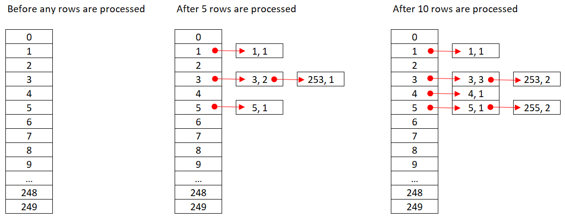
Figure 2: Hash table states
Once the Hash Aggregate operator finishes consuming all input rows, the hash table has all groups with the final state of the aggregate.
Like the Sort operator, the Hash Aggregate operator requires a memory grant, and if it runs out of memory, it needs to spill to tempdb; however, whereas sorting requires a memory grant that is proportional to the number of rows to be sorted, hashing requires a memory grant that is proportional to the number of groups. So especially when the grouping set has high density (small number of groups), this algorithm requires significantly less memory than when explicit sorting is required.
Consider the following two queries (call them Query 1 and Query 2):
SELECT empid, COUNT(*) AS numorders
  FROM dbo.Orders
  GROUP BY empid
  OPTION (HASH GROUP, MAXDOP 1);

SELECT empid, COUNT(*) AS numorders
  FROM dbo.Orders
  GROUP BY empid
  OPTION (ORDER GROUP, MAXDOP 1);
Figure 3 compares the memory grants for these queries.
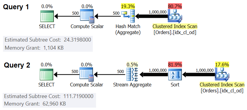
Figure 3: Plans for Query 1 and Query 2
Notice the big difference between the memory grants in the two cases.
As for the Hash Aggregate operator’s cost, going back to Figure 1, notice that there’s no I/O cost, rather only a CPU cost. Next, try to reverse engineer the CPU costing formula using similar techniques to the ones I covered in the previous parts in the series. The factors that can potentially affect the operator’s cost are the number of input rows, number of output groups, the aggregate function used, and what you group by (cardinality of grouping set, data types used).
You’d expect this operator to have a startup cost in preparation for building the hash table. You’d also expect it to scale linearly with respect to the number of rows and groups. That’s indeed what I found. However, whereas the costs of both the Stream Aggregate and Sort operators is not affected by what you group by, it seems that the cost of the Hash Aggregate operator is—both in terms of the cardinality of the grouping set and the data types used.
To observe that the cardinality of the grouping set affects the operator’s cost, check the CPU costs of the Hash Aggregate operators in the plans for the following queries (call them Query 3 and Query 4):
SELECT orderid % 1000 AS grp, MAX(orderdate) AS maxod
  FROM (SELECT TOP (20000) * FROM dbo.Orders) AS D
  GROUP BY orderid % 1000
  OPTION(HASH GROUP, MAXDOP 1);

SELECT orderid % 50 AS grp1, orderid % 20 AS grp2, MAX(orderdate) AS maxod
  FROM (SELECT TOP (20000) * FROM dbo.Orders) AS D
  GROUP BY orderid % 50, orderid % 20
  OPTION(HASH GROUP, MAXDOP 1);
Of course, you want to make sure that the estimated number of input rows and output groups is the same in both cases. The estimated plans for these queries are shown in Figure 4.
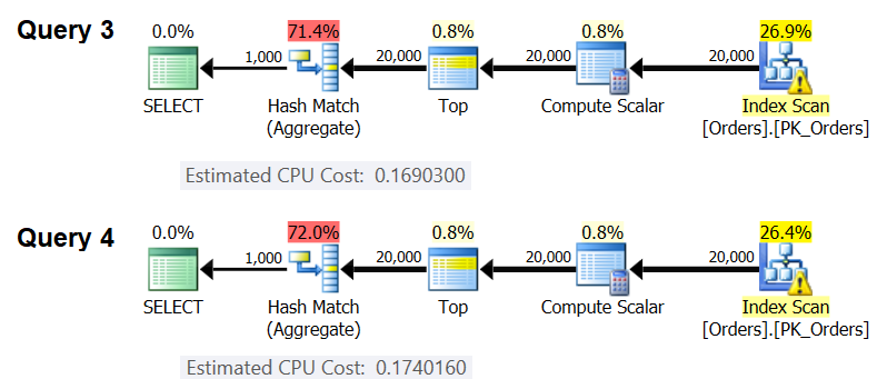
Figure 4: Plans for Query 3 and Query 4
As you can see, the CPU cost of the Hash Aggregate operator is 0.16903 when grouping by one integer column, and 0.174016 when grouping by two integer columns, with all else being equal. This means that the grouping set cardinality indeed affects the cost.
As for whether the data type of the grouped element affects the cost, I used the following queries to check this (call them Query 5, Query 6 and Query 7):
SELECT CAST(orderid AS SMALLINT) % CAST(1000 AS SMALLINT) AS grp,
    MAX(orderdate) AS maxod
  FROM (SELECT TOP (20000) * FROM dbo.Orders) AS D
  GROUP BY CAST(orderid AS SMALLINT) % CAST(1000 AS SMALLINT)
  OPTION(HASH GROUP, MAXDOP 1);

SELECT orderid % 1000 AS grp, MAX(orderdate) AS maxod
  FROM (SELECT TOP (20000) * FROM dbo.Orders) AS D
  GROUP BY orderid % 1000
  OPTION(HASH GROUP, MAXDOP 1);

SELECT CAST(orderid AS BIGINT) % CAST(1000 AS BIGINT) AS grp,
    MAX(orderdate) AS maxod
  FROM (SELECT TOP (20000) * FROM dbo.Orders) AS D
  GROUP BY CAST(orderid AS BIGINT) % CAST(1000 AS BIGINT)
  OPTION(HASH GROUP, MAXDOP 1);
The plans for all three queries have the same estimated number of input rows and output groups, yet they do all get different estimated CPU costs (0.121766, 0.16903 and 0.171716), hence the data type used does affect cost.
The type of aggregate function also seems to have an impact on the cost. For example, consider the following two queries (call them Query 8 and Query 9):
SELECT orderid % 1000 AS grp, COUNT(*) AS numorders
  FROM (SELECT TOP (20000) * FROM dbo.Orders) AS D
  GROUP BY orderid % 1000
  OPTION(HASH GROUP, MAXDOP 1);

SELECT orderid % 1000 AS grp, MAX(orderdate) AS maxod
  FROM (SELECT TOP (20000) * FROM dbo.Orders) AS D
  GROUP BY orderid % 1000
  OPTION(HASH GROUP, MAXDOP 1);
The estimated CPU cost for the Hash Aggregate in the plan for Query 8 is 0.166344, and in Query 9 is 0.16903.
It could be an interesting exercise to try and figure out exactly in what way the cardinality of the grouping set, the data types, and aggregate function used affect the cost; I just didn’t pursue this aspect of the costing. So, after making a choice of the grouping set and aggregate function for your query, you can reverse engineer the costing formula. For example, let’s reverse engineer the CPU costing formula for the Hash Aggregate operator when grouping by a single integer column and returning the MAX(orderdate) aggregate. The formula should be:
Using the techniques that I demonstrated in the previous articles in the series, I got the following reverse engineered formula:
You can check the accuracy of the formula using the following queries:
SELECT orderid % 1000 AS grp, MAX(orderdate) AS maxod
  FROM (SELECT TOP (100000) * FROM dbo.Orders) AS D
  GROUP BY orderid % 1000
  OPTION(HASH GROUP, MAXDOP 1);

SELECT orderid % 2000 AS grp, MAX(orderdate) AS maxod
  FROM (SELECT TOP (100000) * FROM dbo.Orders) AS D
  GROUP BY orderid % 2000
  OPTION(HASH GROUP, MAXDOP 1);

SELECT orderid % 3000 AS grp, MAX(orderdate) AS maxod
  FROM (SELECT TOP (200000) * FROM dbo.Orders) AS D
  GROUP BY orderid % 3000
  OPTION(HASH GROUP, MAXDOP 1);

SELECT orderid % 6000 AS grp, MAX(orderdate) AS maxod
  FROM (SELECT TOP (200000) * FROM dbo.Orders) AS D
  GROUP BY orderid % 6000
  OPTION(HASH GROUP, MAXDOP 1);

SELECT orderid % 5000 AS grp, MAX(orderdate) AS maxod
  FROM (SELECT TOP (500000) * FROM dbo.Orders) AS D
  GROUP BY orderid % 5000
  OPTION(HASH GROUP, MAXDOP 1);

SELECT orderid % 10000 AS grp, MAX(orderdate) AS maxod
  FROM (SELECT TOP (500000) * FROM dbo.Orders) AS D
  GROUP BY orderid % 10000
  OPTION(HASH GROUP, MAXDOP 1);
I get the following results:
numrows     numgroups   predictedcost  estimatedcost
----------- ----------- -------------- --------------
100000      1000        0.703315       0.703316
100000      2000        0.721023       0.721024
200000      3000        1.40659        1.40659
200000      6000        1.45972        1.45972
500000      5000        3.44558        3.44558
500000      10000       3.53412        3.53412
The formula seems to be spot on.
Costing summary and comparison
Now we have the costing formulas for the three available strategies: preordered Stream Aggregate, Sort + Stream Aggregate and Hash Aggregate. The following table summarizes and compares the costing characteristics of the three algorithms:
|
Preordered Stream Aggregate |
Sort + Stream Aggregate |
Hash Aggregate |
|
|
Formula |
@numrows * 0.0000006 + @numgroups * 0.0000005 |
0.0112613 +
Small number of rows: 9.99127891201865E-05 + @numrows * LOG(@numrows) * 2.25061348918698E-06 Large number of rows: 1.35166186417734E-04 + @numrows * LOG(@numrows) * 6.62193536908588E-06 + @numrows * 0.0000006 + @numgroups * 0.0000005 |
0.017749 + @numrows * 0.00000667857 + @numgroups * 0.0000177087 * Grouping by single integer column, returning MAX(<date column>) |
|
Scaling |
linear | n log n | linear |
|
Startup I/O cost |
none | 0.0112613 | none |
|
Startup CPU cost |
none | ~ 0.0001 | 0.017749 |
According to these formulas, Figure 5 shows the way each of the strategies scales for different numbers of input rows, using a fixed number of groups of 500 as an example.
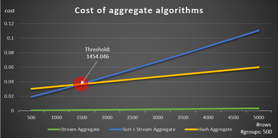
Figure 5: Cost of aggregate algorithms
You can clearly see that if the data is preordered, e.g., in a covering index, the preordered Stream Aggregate strategy is the best option, irrespective of how many rows are involved. For example, suppose that you need to query the Orders table, and compute the maximum order date for each employee. You create the following covering index:
CREATE INDEX idx_eid_od ON dbo.Orders(empid, orderdate);Here are five queries, emulating an Orders table with different numbers of rows (10,000, 20,000, 30,000, 40,000 and 50,000):
SELECT empid, MAX(orderdate) AS maxod
  FROM (SELECT TOP (10000) * FROM dbo.Orders) AS D
  GROUP BY empid;

SELECT empid, MAX(orderdate) AS maxod
  FROM (SELECT TOP (20000) * FROM dbo.Orders) AS D
  GROUP BY empid;

SELECT empid, MAX(orderdate) AS maxod
  FROM (SELECT TOP (30000) * FROM dbo.Orders) AS D
  GROUP BY empid;

SELECT empid, MAX(orderdate) AS maxod
  FROM (SELECT TOP (40000) * FROM dbo.Orders) AS D
  GROUP BY empid;

SELECT empid, MAX(orderdate) AS maxod
  FROM (SELECT TOP (50000) * FROM dbo.Orders) AS D
  GROUP BY empid;
Figure 6 shows the plans for these queries.
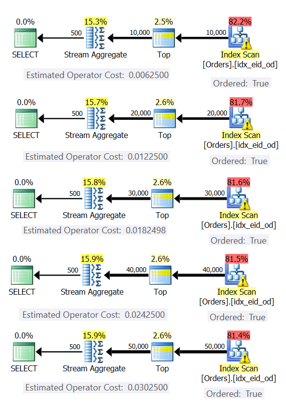
Figure 6: Plans with preordered Stream Aggregate strategy
In all cases, the plans perform an ordered scan of the covering index, and apply the Stream Aggregate operator without the need for explicit sorting.
Use the following code to drop the index you created for this example:
DROP INDEX idx_eid_od ON dbo.Orders;The other important thing to note about the graphs in Figure 5 is what happens when the data is not preordered. This happens when there’s no covering index in place, as well as when you group by manipulated expressions as opposed to base columns. There is an optimization threshold—in our case at 1454.046 rows—below which the Sort + Stream Aggregate strategy has a lower cost, and on or above which the Hash Aggregate strategy has a lower cost. This has to do with the fact that the former hash a lower startup cost, but scales in an n log n manner, whereas the latter has a higher startup cost but scales linearly. This makes the former preferred with small numbers of input rows. If our reverse engineered formulas are accurate, the following two queries (call them Query 10 and Query 11) should get different plans:
SELECT orderid % 500 AS grp, MAX(orderdate) AS maxod
  FROM (SELECT TOP (1454) * FROM dbo.Orders) AS D
  GROUP BY orderid % 500;

SELECT orderid % 500 AS grp, MAX(orderdate) AS maxod
  FROM (SELECT TOP (1455) * FROM dbo.Orders) AS D
  GROUP BY orderid % 500;
The plans for these queries are shown in Figure 7.
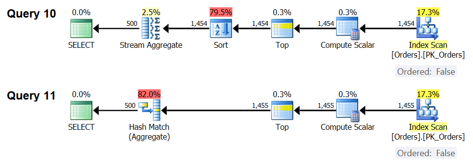
Figure 7: Plans for Query 10 and Query 11
Indeed, with 1,454 input rows (below the optimization threshold), the optimizer naturally prefers the Sort + Stream Aggregate algorithm for Query 10, and with 1,455 input rows (above the optimization threshold), the optimizer naturally prefers the Hash Aggregate algorithm for Query 11.
Potential for Adaptive Aggregate operator
One of the tricky aspects of optimization thresholds is parameter-sniffing problems when using parameter-sensitive queries in stored procedures. Consider the following stored procedure as an example:
CREATE OR ALTER PROC dbo.EmpOrders
  @initialorderid AS INT
AS
  SELECT empid, COUNT(*) AS numorders
  FROM dbo.Orders
  WHERE orderid >= @initialorderid
  GROUP BY empid;
GO
You create the following optimal index to support the stored procedure query:
CREATE INDEX idx_oid_i_eid ON dbo.Orders(orderid) INCLUDE(empid);You created the index with orderid as the key to support the query’s range filter, and included empid for coverage. This is a situation where you can’t really create an index that will both support the range filter and have the filtered rows preordered by the grouping set. This means that the optimizer will have to make a choice between the Sort + stream Aggregate and the Hash Aggregate algorithms. Based on our costing formulas, the optimization threshold is between 937 and 938 input rows (let’s say, 937.5 rows).
Suppose that you execute the stored procedure first time with an input initial order ID that gives you a small number of matches (below the threshold):
EXEC dbo.EmpOrders @initialorderid = 999991;SQL Server produces a plan that uses the Sort + Stream Aggregate algorithm, and caches the plan. Subsequent executions reuse the cached plan, irrespective of how many rows are involved. For instance, the following execution has a number of matches above the optimization threshold:
EXEC dbo.EmpOrders @initialorderid = 990001;Still, it reuses the cached plan despite the fact that it’s not optimal for this execution. That’s a classic parameter sniffing problem.
SQL Server 2017 introduces adaptive query processing capabilities, which are designed to cope with such situations by determining during query execution which strategy to employ. Among those improvements is an Adaptive Join operator which during execution determines whether to activate a Loop or Hash algorithm based on a computed optimization threshold. Our aggregate story begs for a similar Adaptive Aggregate operator, which during execution would make a choice between a Sort + Stream Aggregate strategy and a Hash Aggregate strategy, based on a computed optimization threshold. Figure 8 illustrates a pseudo plan based on this idea.
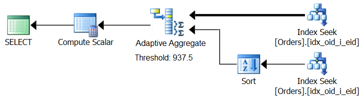
Figure 8: Pseudo plan with Adaptive Aggregate operator
For now, in order to get such a plan you need to use Microsoft Paint. But since the concept of adaptive query processing is so smart and works so well, it’s only reasonable to expect to see further improvements in this area in the future.
Run the following code to drop the index you created for this example:
DROP INDEX idx_oid_i_eid ON dbo.Orders;Conclusion
In this article I covered the costing and scaling of the Hash Aggregate algorithm and compared it with the Stream Aggregate and Sort + Stream Aggregate strategies. I described the optimization threshold that exists between the Sort + Stream Aggregate and Hash Aggregate strategies. With small numbers of input rows the former is preferred and with large numbers the latter. I also described the potential for adding an Adaptive Aggregate operator, similar to the already implemented Adaptive Join operator, to help deal with parameter-sniffing problems when using parameter-sensitive queries. Next month I’ll continue the discussion by covering parallelism considerations and cases that call for query rewrites.
10 thoughts on “Optimization Thresholds – Grouping and Aggregating Data, Part 3”
Comments are closed.
Love your comment "For now, in order to get such a plan you need to use Microsoft Paint", Itzik!
That’s what I used. :)
CREATE INDEX idx_oid_i_eid ON dbo.Orders(orderid) INCLUDE(empid);
If i Create Index as
CREATE INDEX idx_oid_i_eid ON dbo.Orders(orderid,empid)
is it better ?
Since the query has a range filter based on orderid, the filtered rows will not be ordered by empid across the filtered range, even if you do make empid the second key column. Therefore, it doesn't matter if you make it a key column or an included column. You just want it there for coverage.
If you had an equality filter, e.g., WHERE shipperid = 'A', then it would have been recommended to place the grouped column as a second key (shipperid, empid), and not as an included column.
Is there any other way to encourage use hash group without using hint?
Hi Pei,
Your question implies that you have situations where the optimizer chooses stream aggregate even though it's not optimal or preferred by you. Can you elaborate on why you're looking for an alternative to a hint? If it's a matter of the optimizer making a suboptimal choice, a typical cause is inaccurate cardinality estimates. In such a case you'd want to investigate a solution that would improve those estimates. If it's a matter of a parameter-sensitive query/a parameter sniffing issue, there are solutions for this as well. But if your goal is to very specifically to force a hash aggregate for some reason, the tool is either a hint specific for this purpose or to force an entire plan either through a plan guide or query store.
Itzik, there are situation such as views, functions where you can not use hint. Also hint is at query level, I think you can not plug in sub query level, and it forces entire query using hash group like force order hint. these queries I worked on did not involved parameter sniffing or stats out of date issues. Some were column store index tables, which is well known that intends to use steam aggregation. I am wondering if row goal (top) strategy could play the trick to encourage hash group.
I hear you. Just like we have individual join hints, would be nice to have individual group hints and not just query level ones. You are allowed to use individual join hints in inner queries used in table expressions like views.
If you’re experiencing inappropriate choices of a stream aggregate algorithm with columnstore (meaning there’s also a sort involved since columnstore isn’t ordered), that’s usually the result of a cardinality under estimation. You say that it’s not an issue with stats, but if indeed it is an under estimation, the root cause should be investigated.
One trick that can affect row goals is to use a combination of a TOP filter with a variable and an OPTIMIZE FOR hint, but this one can reduce the original estimate and not increase it, and in order to get a hash aggregate strategy, you typically need a higher estimate than the original one that resulted in the use of the stream aggregate strategy. Also, variables are not allowed in views, so in order to use a parameter, you would need to convert the view to an inline TVF. In short, I don’t see an easy way to encourage an individual group hash aggregate.
Plus, the OPTIMIZE FOR hint is a query option, so anyway you cannot use it in an inner query, rather you'd have to use it in the outer query against the table expression.
Itzik,
Thank you for your reply. I think the conclusion is that there is no easy way to encourage an individual group hash aggregate. Additionally clustered columnstore tables do not have stats other than individual columns based on info returned from sys.dm_db_stats_properties.