Last month, I covered Peter Larsson's puzzle of matching supply with demand. I showed Peter's straightforward cursor-based solution and explained that it has linear scaling. The challenge I left you with is to try and come up with a set-based solution to the task, and boy, have people risen to the challenge! Thanks Luca, Kamil Kosno, Daniel Brown, Brian Walker, Joe Obbish, Rainer Hoffmann, Paul White, Charlie, and, of course, Peter Larsson, for sending your solutions. Some of the ideas were brilliant and outright mind-blowing.
This month, I'm going to start exploring the submitted solutions, roughly, going from the worse performing to the best performing ones. Why even bother with the bad performing ones? Because you can still learn a lot from them; for example, by identifying anti-patterns. Indeed, the first attempt at solving this challenge for many people, including myself and Peter, is based on an interval intersection concept. It so happens that the classic predicate-based technique for identifying interval intersection has poor performance since there's no good indexing scheme to support it. This article is dedicated to this poor performing approach. Despite the poor performance, working on the solution is an interesting exercise. It requires practicing the skill of modeling the problem in a way that lends itself to set-based treatment. It is also interesting to identify the reason for the bad performance, making it easier to avoid the anti-pattern in the future. Keep in mind, this solution is just the starting point.
DDL and a Small Set of Sample Data
As a reminder, the task involves querying a table called "Auctions."" Use the following code to create the table and populate it with a small set of sample data:
DROP TABLE IF EXISTS dbo.Auctions;

CREATE TABLE dbo.Auctions
(
  ID INT NOT NULL IDENTITY(1, 1)
    CONSTRAINT pk_Auctions PRIMARY KEY CLUSTERED,
  Code CHAR(1) NOT NULL
    CONSTRAINT ck_Auctions_Code CHECK (Code = 'D' OR Code = 'S'),
  Quantity DECIMAL(19, 6) NOT NULL
    CONSTRAINT ck_Auctions_Quantity CHECK (Quantity > 0)
);

SET NOCOUNT ON;

DELETE FROM dbo.Auctions;

SET IDENTITY_INSERT dbo.Auctions ON;

INSERT INTO dbo.Auctions(ID, Code, Quantity) VALUES
  (1, 'D', 5.0),
  (2, 'D', 3.0),
  (3, 'D', 8.0),
  (5, 'D', 2.0),
  (6, 'D', 8.0),
  (7, 'D', 4.0),
  (8, 'D', 2.0),
  (1000, 'S', 8.0),
  (2000, 'S', 6.0),
  (3000, 'S', 2.0),
  (4000, 'S', 2.0),
  (5000, 'S', 4.0),
  (6000, 'S', 3.0),
  (7000, 'S', 2.0);

SET IDENTITY_INSERT dbo.Auctions OFF;
Your task was to create pairings that match supply with demand entries based on ID ordering, writing those to a temporary table. Following is the desired result for the small set of sample data:
DemandID    SupplyID    TradeQuantity
----------- ----------- --------------
1           1000        5.000000
2           1000        3.000000
3           2000        6.000000
3           3000        2.000000
5           4000        2.000000
6           5000        4.000000
6           6000        3.000000
6           7000        1.000000
7           7000        1.000000
Last month, I also provided code that you can use to populate the Auctions table with a large set of sample data, controlling the number of supply and demand entries as well as their range of quantities. Make sure that you use the code from last month's article to check the performance of the solutions.
Modeling the Data as Intervals
One intriguing idea that lends itself to supporting set-based solutions is to model the data as intervals. In other words, represent each demand and supply entry as an interval starting with the running total quantities of the same kind (demand or supply) up to but excluding the current, and ending with the running total including the current, of course based on ID ordering. For example, looking at the small set of sample data, the first demand entry (ID 1) is for a quantity of 5.0 and the second (ID 2) is for a quantity of 3.0. The first demand entry can be represented with the interval start: 0.0, end: 5.0, and the second with the interval start: 5.0, end: 8.0, and so on.
Similarly, the first supply entry (ID 1000) is for a quantity of 8.0 and the second (ID 2000) is for a quantity of 6.0. The first supply entry can be represented with the interval start: 0.0, end: 8.0, and the second with the interval start: 8.0, end: 14.0, and so on.
The demand-supply pairings you need to create are then the overlapping segments of the intersecting intervals between the two kinds.
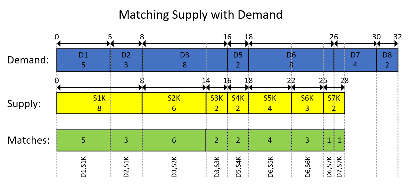
This is probably best understood with a visual depiction of the interval-based modeling of the data and the desired result, as shown in Figure 1.
 Figure 1: Modeling the Data as Intervals
The visual depiction in Figure 1 is pretty self-explanatory but, in short…
The blue rectangles represent the demand entries as intervals, showing the exclusive running total quantities as the start of the interval and the inclusive running total as the end of the interval. The yellow rectangles do the same for supply entries. Then notice how the overlapping segments of the intersecting intervals of the two kinds, which are depicted by the green rectangles, are the demand-supply pairings you need to produce. For example, the first result pairing is with demand ID 1, supply ID 1000, quantity 5. The second result pairing is with demand ID 2, supply ID 1000, quantity 3. And so on.
Interval Intersections Using CTEs
Before you start writing the T-SQL code with solutions based on the interval modeling idea, you should already have an intuitive sense for what indexes are likely to be useful here. Since you're likely to use window functions to compute running totals, you could benefit from a covering index with a key based on the columns Code, ID, and including the column Quantity. Here's the code to create such an index:
CREATE UNIQUE NONCLUSTERED INDEX idx_Code_ID_i_Quantity
  ON dbo.Auctions(Code, ID)
  INCLUDE(Quantity);
That's the same index I recommended for the cursor-based solution that I covered last month.
Also, there's potential here to benefit from batch processing. You can enable its consideration without the requirements of batch mode on rowstore, e.g., using SQL Server 2019 Enterprise or later, by creating the following dummy columnstore index:
CREATE NONCLUSTERED COLUMNSTORE INDEX idx_cs
  ON dbo.Auctions(ID)
  WHERE ID = -1 AND ID = -2;
You can now start working on the solution's T-SQL code.
The following code creates the intervals representing the demand entries:
WITH D0 AS
-- D0 computes running demand as EndDemand
(
  SELECT ID, Quantity,
    SUM(Quantity) OVER(ORDER BY ID ROWS UNBOUNDED PRECEDING) AS EndDemand
  FROM dbo.Auctions
  WHERE Code = 'D'
),
-- D extracts prev EndDemand as StartDemand, expressing start-end demand as an interval
D AS
(
  SELECT ID, Quantity, EndDemand - Quantity AS StartDemand, EndDemand
  FROM D0
)
SELECT *
FROM D;
The query defining the CTE D0 filters demand entries from the Auctions table and computes a running total quantity as the end delimiter of the demand intervals. Then the query defining the second CTE called D queries D0 and computes the start delimiter of the demand intervals by subtracting the current quantity from the end delimiter.
This code generates the following output:
ID   Quantity  StartDemand  EndDemand
---- --------- ------------ ----------
1    5.000000  0.000000     5.000000
2    3.000000  5.000000     8.000000
3    8.000000  8.000000     16.000000
5    2.000000  16.000000    18.000000
6    8.000000  18.000000    26.000000
7    4.000000  26.000000    30.000000
8    2.000000  30.000000    32.000000
The supply intervals are generated very similarly by applying the same logic to the supply entries, using the following code:
WITH S0 AS
-- S0 computes running supply as EndSupply
(
  SELECT ID, Quantity,
    SUM(Quantity) OVER(ORDER BY ID ROWS UNBOUNDED PRECEDING) AS EndSupply
  FROM dbo.Auctions
  WHERE Code = 'S'
),
-- S extracts prev EndSupply as StartSupply, expressing start-end supply as an interval
S AS
(
  SELECT ID, Quantity, EndSupply - Quantity AS StartSupply, EndSupply
  FROM S0
)
SELECT *
FROM S;
This code generates the following output:
ID    Quantity  StartSupply  EndSupply
----- --------- ------------ ----------
1000  8.000000  0.000000     8.000000
2000  6.000000  8.000000     14.000000
3000  2.000000  14.000000    16.000000
4000  2.000000  16.000000    18.000000
5000  4.000000  18.000000    22.000000
6000  3.000000  22.000000    25.000000
7000  2.000000  25.000000    27.000000
What's left is then to identify the intersecting demand and supply intervals from the CTEs D and S, and compute the overlapping segments of those intersecting intervals. Remember the result pairings should be written into a temporary table. This can be done using the following code:
-- Drop temp table if exists
DROP TABLE IF EXISTS #MyPairings;

WITH D0 AS
-- D0 computes running demand as EndDemand
(
  SELECT ID, Quantity,
    SUM(Quantity) OVER(ORDER BY ID ROWS UNBOUNDED PRECEDING) AS EndDemand
  FROM dbo.Auctions
  WHERE Code = 'D'
),
-- D extracts prev EndDemand as StartDemand, expressing start-end demand as an interval
D AS
(
  SELECT ID, Quantity, EndDemand - Quantity AS StartDemand, EndDemand
  FROM D0
),
S0 AS
-- S0 computes running supply as EndSupply
(
  SELECT ID, Quantity,
    SUM(Quantity) OVER(ORDER BY ID ROWS UNBOUNDED PRECEDING) AS EndSupply
  FROM dbo.Auctions
  WHERE Code = 'S'
),
-- S extracts prev EndSupply as StartSupply, expressing start-end supply as an interval
S AS
(
  SELECT ID, Quantity, EndSupply - Quantity AS StartSupply, EndSupply
  FROM S0
)
-- Outer query identifies trades as the overlapping segments of the intersecting intervals
-- In the intersecting demand and supply intervals the trade quantity is then
-- LEAST(EndDemand, EndSupply) - GREATEST(StartDemsnad, StartSupply)
SELECT
  D.ID AS DemandID, S.ID AS SupplyID,
  CASE WHEN EndDemand < EndSupply THEN EndDemand ELSE EndSupply END - CASE WHEN StartDemand > StartSupply THEN StartDemand ELSE StartSupply END
    AS TradeQuantity
INTO #MyPairings
FROM D INNER JOIN S
  ON D.StartDemand < S.EndSupply AND D.EndDemand > S.StartSupply;
Besides the code that creates the demand and supply intervals, which you already saw earlier, the main addition here is the outer query, which identifies the intersecting intervals between D and S, and computes the overlapping segments. To identify the intersecting intervals, the outer query joins D and S using the following join predicate:
D.StartDemand < S.EndSupply AND D.EndDemand > S.StartSupply
That's the classic predicate to identify interval intersection. It's also the main source for the solution's poor performance, as I'll explain shortly.
The outer query also computes the trade quantity in the SELECT list as:
LEAST(EndDemand, EndSupply) - GREATEST(StartDemand, StartSupply)
If you're using Azure SQL, you can use this expression. If you're using SQL Server 2019 or earlier, you can use the following logically equivalent alternative:
CASE WHEN EndDemand < EndSupply THEN EndDemand ELSE EndSupply END - CASE WHEN StartDemand > StartSupply THEN StartDemand ELSE StartSupply END
Since the requirement was to write the result into a temporary table, the outer query uses a SELECT INTO statement to achieve this.
The idea to model the data as intervals is clearly intriguing and elegant. But what about performance? Unfortunately, this specific solution has a big problem related to how interval intersection is identified. Examine the plan for this solution shown in Figure 2.
 Figure 2: Query Plan for Intersections Using CTEs Solution
Let's start with the inexpensive parts of the plan.
The outer input of the Nested Loops join computes the demand intervals. It uses an Index Seek operator to retrieve the demand entries, and a batch mode Window Aggregate operator to compute the demand interval end delimiter (referred to as Expr1005 in this plan). The demand interval start delimiter is then Expr1005 – Quantity (from D).
As a side note, you might find the use of an explicit Sort operator prior to the batch mode Window Aggregate operator surprising here, since the demand entries retrieved from the Index Seek are already ordered by ID like the window function needs them to be. This has to do with the fact that currently, SQL Server doesn't support an efficient combination of parallel order-preserving index operation prior to a parallel batch mode Window Aggregate operator. If you force a serial plan just for experimentation purposes, you'll see the Sort operator disappearing. SQL Server decided overall, the use of parallelism here was preferred, despite it resulting in the added explicit sorting. But again, this part of the plan represents a small portion of the work in the grand scheme of things.
Similarly, the inner input of the Nested Loops join starts by computing the supply intervals. Curiously, SQL Server chose to use row-mode operators to handle this part. On one hand, row mode operators used to compute running totals involve more overhead than the batch mode Window Aggregate alternative; on the other hand, SQL Server has an efficient parallel implementation of an order-preserving index operation following by the window function's computation, avoiding explicit Sorting for this part. It's curious the optimizer chose one strategy for the demand intervals and another for the supply intervals. At any rate, the Index Seek operator retrieves the supply entries, and the subsequent sequence of operators up to the Compute Scalar operator compute the supply interval end delimiter (referred to as Expr1009 in this plan). The supply interval start delimiter is then Expr1009 – Quantity (from S).
Despite the amount of text I used to describe these two parts, the truly expensive part of the work in the plan is what comes next.
The next part needs to join the demand intervals and the supply intervals using the following predicate:
D.StartDemand < S.EndSupply AND D.EndDemand > S.StartSupply
With no supporting index, assuming DI demand intervals and SI supply intervals, this would involve processing DI * SI rows. The plan in Figure 2 was created after filling the Auctions table with 400,000 rows (200,000 demand entries and 200,000 supply entries). So, with no supporting index, the plan would have needed to process 200,000 * 200,000 = 40,000,000,000 rows. To mitigate this cost, the optimizer chose to create a temporary index (see the Index Spool operator) with the supply interval end delimiter (Expr1009) as the key. That's pretty much the best it could do. However, this takes care of only part of the problem. With two range predicates, only one can be supported by an index seek predicate. The other has to be handled using a residual predicate. Indeed, you can see in the plan that the seek in the temporary index uses the seek predicate Expr1009 > Expr1005 – D.Quantity, followed by a Filter operator handling the residual predicate Expr1005 > Expr1009 – S.Quantity.
Assuming on average, the seek predicate isolates half the supply rows from the index per demand row, the total number of rows emitted from the Index Spool operator and processed by the Filter operator is then DI * SI / 2. In our case, with 200,000 demand rows and 200,000 supply rows, this translates to 20,000,000,000. Indeed, the arow going from the Index Spool operator to the Filter operator reports a number of rows close to this.
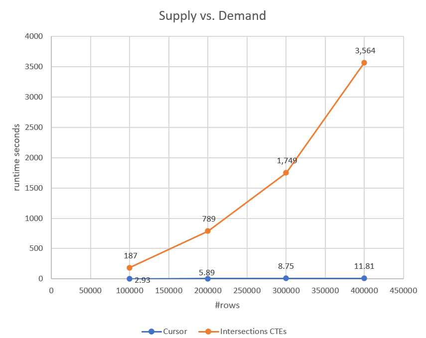
This plan has quadratic scaling, compared to the linear scaling of the cursor-based solution from last month. You can see the result of a performance test comparing the two solutions in Figure 3. You can clearly see the nicely shaped parabola for the set-based solution.
 Figure 3: Performance of Intersections Using CTEs Solution Versus Cursor-Based Solution
Interval Intersections Using Temporary Tables
You can somewhat improve things by replacing the use of CTEs for the demand and supply intervals with temporary tables, and to avoid the index spool, creating your own index on the temp table holding the supply intervals with the end delimiter as the key. Here's the complete solution's code:
-- Drop temp tables if exist
DROP TABLE IF EXISTS #MyPairings, #Demand, #Supply;

WITH D0 AS
-- D0 computes running demand as EndDemand
(
  SELECT ID, Quantity,
    SUM(Quantity) OVER(ORDER BY ID ROWS UNBOUNDED PRECEDING) AS EndDemand
  FROM dbo.Auctions
  WHERE Code = 'D'
),
-- D extracts prev EndDemand as StartDemand, expressing start-end demand as an interval
D AS
(
  SELECT ID, Quantity, EndDemand - Quantity AS StartDemand, EndDemand
  FROM D0
)
SELECT ID, Quantity,
  CAST(ISNULL(StartDemand, 0.0) AS DECIMAL(19, 6)) AS StartDemand,
  CAST(ISNULL(EndDemand, 0.0) AS DECIMAL(19, 6)) AS EndDemand
INTO #Demand
FROM D;
WITH S0 AS
-- S0 computes running supply as EndSupply
(
  SELECT ID, Quantity,
    SUM(Quantity) OVER(ORDER BY ID ROWS UNBOUNDED PRECEDING) AS EndSupply
  FROM dbo.Auctions
  WHERE Code = 'S'
),
-- S extracts prev EndSupply as StartSupply, expressing start-end supply as an interval
S AS
(
  SELECT ID, Quantity, EndSupply - Quantity AS StartSupply, EndSupply
  FROM S0
)
SELECT ID, Quantity,
  CAST(ISNULL(StartSupply, 0.0) AS DECIMAL(19, 6)) AS StartSupply,
  CAST(ISNULL(EndSupply, 0.0) AS DECIMAL(19, 6)) AS EndSupply
INTO #Supply
FROM S;

CREATE UNIQUE CLUSTERED INDEX idx_cl_ES_ID ON #Supply(EndSupply, ID);

-- Outer query identifies trades as the overlapping segments of the intersecting intervals
-- In the intersecting demand and supply intervals the trade quantity is then
-- LEAST(EndDemand, EndSupply) - GREATEST(StartDemsnad, StartSupply)
SELECT
  D.ID AS DemandID, S.ID AS SupplyID,
  CASE WHEN EndDemand < EndSupply THEN EndDemand ELSE EndSupply END - CASE WHEN StartDemand > StartSupply THEN StartDemand ELSE StartSupply END
    AS TradeQuantity
INTO #MyPairings
FROM #Demand AS D
  INNER JOIN #Supply AS S WITH (FORCESEEK)
    ON D.StartDemand < S.EndSupply AND D.EndDemand > S.StartSupply;
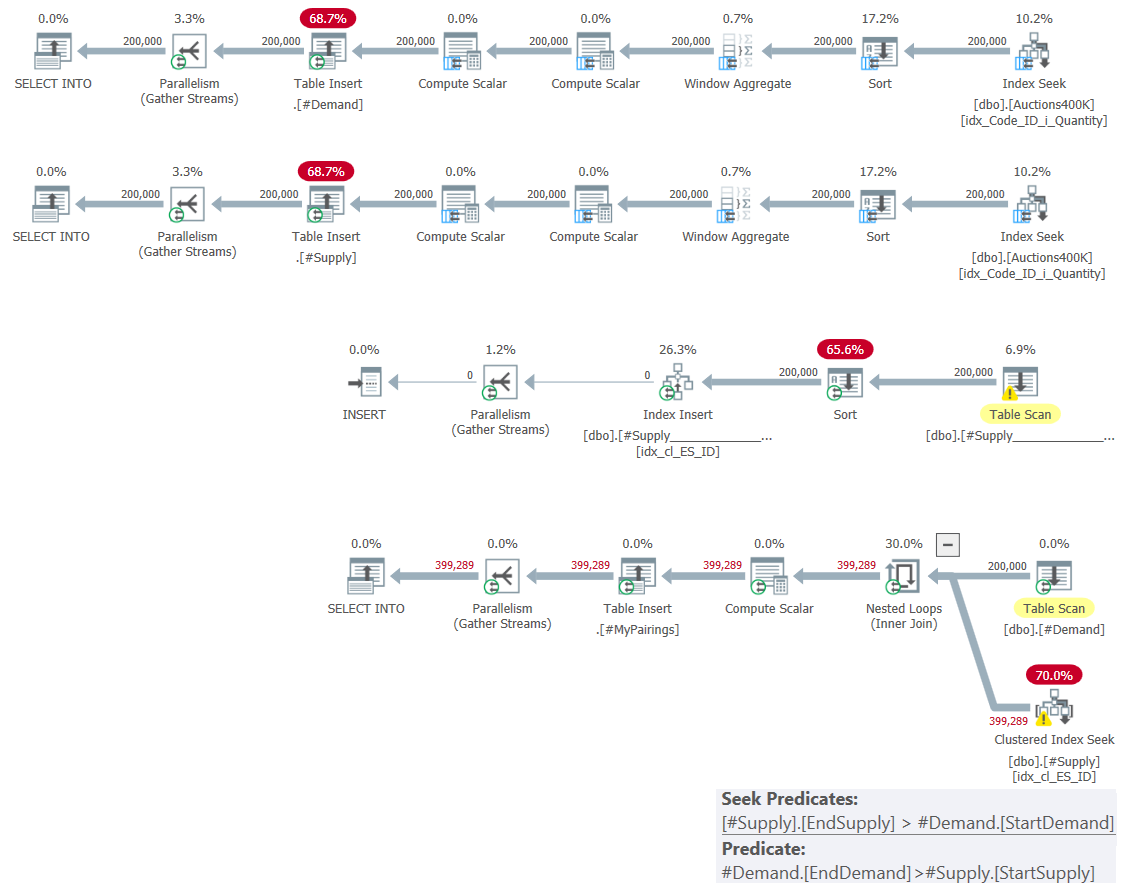
The plans for this solution are shown in Figure 4:
 Figure 4: Query Plan for Intersections Using Temp Tables Solution
The first two plans use a combination of batch-mode Index Seek + Sort + Window Aggregate operators to compute the supply and demand intervals and write those to temporary tables. The third plan handles the index creation on the #Supply table with the EndSupply delimiter as the leading key.
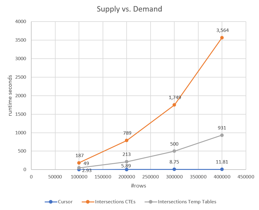
The fourth plan represents by far the bulk of the work, with a Nested Loops join operator that matches to each interval from #Demand, the intersecting intervals from #Supply. Observe that also here, the Index Seek operator relies on the predicate #Supply.EndSupply > #Demand.StartDemand as the seek predicate, and #Demand.EndDemand > #Supply.StartSupply as the residual predicate. So in terms of complexity/scaling, you get the same quadratic complexity like for the previous solution. You just pay less per row since you're using your own index instead of the index spool used by the previous plan. You can see the performance of this solution compared to the previous two in Figure 5.
 Figure 5: Performance of Intersections using temp tables compared to other two solutions
As you can see, the solution with the temp tables performs better than the one with the CTEs, but it still has quadratic scaling and does very badly compared to the cursor.
What's Next?
This article covered the first attempt at handling the classic matching supply with demand task using a set-based solution. The idea was to model the data as intervals, match supply with demand entries by identifying intersecting supply and demand intervals, and then compute the trading quantity based on the size of the overlapping segments. Certainly an intriguing idea. The main problem with it is also the classic problem of identifying interval intersection by using two range predicates. Even with the best index in place, you can only support one range predicate with an index seek; the other range predicate has to be handled using a residual predicate. This results in a plan with quadratic complexity.
So what can you do to overcome this obstacle? There are several different ideas. One brilliant idea belongs to Joe Obbish, which you can read about in detail in his blog post. I'll cover other ideas in upcoming articles in the series.


I had a feeling that solution is going to be slow. I wasn't able to test it properly on a large dataset.
With a small amount of rows, I reckon it's probably the most straightforward option we're going to see
You will have to be patient. There are more to show! :-)