
Matching Supply With Demand — Solutions, Part 3
In this article, I continue exploring solutions to the matching supply with demand challenge. Thanks to Luca, Kamil Kosno, Daniel Brown, Brian Walker, Joe Obbish, Rainer Hoffmann, Paul White, Charlie, Ian, and Peter Larsson, for sending your solutions.
Last month I covered solutions based on a revised interval intersections approach compared to the classic one. The fastest of those solutions combined ideas from Kamil, Luca, and Daniel. It unified two queries with disjoint sargable predicates. It took the solution 1.34 seconds to complete against a 400K-row input. That’s not too shabby considering the solution based on the classic interval intersections approach took 931 seconds to complete against the same input. Also recall Joe came up with a brilliant solution that relies on the classic interval intersection approach but optimizes the matching logic by bucketizing intervals based on the largest interval length. With the same 400K-row input, it took Joe’s solution 0.9 seconds to complete. The tricky part about this solution is its performance degrades as the largest interval length increases.
This month I explore fascinating solutions that are faster than the Kamil/Luca/Daniel Revised Intersections solution and are neutral to interval length. The solutions in this article were created by Brian Walker, Ian, Peter Larsson, Paul White, and me.
I tested all solutions in this article against the Auctions input table with 100K, 200K, 300K, and 400K rows, and with the following indexes:
-- Index to support solution

CREATE UNIQUE NONCLUSTERED INDEX idx_Code_ID_i_Quantity
  ON dbo.Auctions(Code, ID)
  INCLUDE(Quantity);

-- Enable batch-mode Window Aggregate

CREATE NONCLUSTERED COLUMNSTORE INDEX idx_cs
  ON dbo.Auctions(ID)
  WHERE ID = -1 AND ID = -2;
When describing the logic behind the solutions, I’ll assume the Auctions table is populated with the following small set of sample data:
ID          Code Quantity
----------- ---- ---------
1           D    5.000000
2           D    3.000000
3           D    8.000000
5           D    2.000000
6           D    8.000000
7           D    4.000000
8           D    2.000000
1000        S    8.000000
2000        S    6.000000
3000        S    2.000000
4000        S    2.000000
5000        S    4.000000
6000        S    3.000000
7000        S    2.000000
Following is the desired result for this sample data:
DemandID    SupplyID    TradeQuantity
----------- ----------- --------------
1           1000        5.000000
2           1000        3.000000
3           2000        6.000000
3           3000        2.000000
5           4000        2.000000
6           5000        4.000000
6           6000        3.000000
6           7000        1.000000
7           7000        1.000000
Brian Walker’s Solution
Outer joins are fairly commonly used in SQL querying solutions, but by far when you use those, you use single-sided ones. When teaching about outer joins, I often get questions asking for examples for practical use cases of full outer joins, and there aren’t that many. Brian’s solution is a beautiful example of a practical use case of full outer joins.
Here’s Brian’s complete solution code:
DROP TABLE IF EXISTS #MyPairings;

CREATE TABLE #MyPairings
(
  DemandID       INT            NOT NULL,
  SupplyID       INT            NOT NULL,
  TradeQuantity  DECIMAL(19,06) NOT NULL
);

WITH D AS
(
  SELECT A.ID,
    SUM(A.Quantity) OVER (PARTITION BY A.Code
                          ORDER BY A.ID ROWS UNBOUNDED PRECEDING) AS Running
  FROM dbo.Auctions AS A
  WHERE A.Code = 'D'
),
S AS
(
  SELECT A.ID,
    SUM(A.Quantity) OVER (PARTITION BY A.Code
                          ORDER BY A.ID ROWS UNBOUNDED PRECEDING) AS Running
  FROM dbo.Auctions AS A
  WHERE A.Code = 'S'
),
W AS
(
  SELECT D.ID AS DemandID, S.ID AS SupplyID, ISNULL(D.Running, S.Running) AS Running
  FROM D
    FULL JOIN S
      ON D.Running = S.Running
),
Z AS
(
  SELECT
    CASE
      WHEN W.DemandID IS NOT NULL THEN W.DemandID
      ELSE MIN(W.DemandID) OVER (ORDER BY W.Running
                                 ROWS BETWEEN CURRENT ROW AND UNBOUNDED FOLLOWING)
    END AS DemandID,
    CASE
      WHEN W.SupplyID IS NOT NULL THEN W.SupplyID
      ELSE MIN(W.SupplyID) OVER (ORDER BY W.Running
                                 ROWS BETWEEN CURRENT ROW AND UNBOUNDED FOLLOWING)
    END AS SupplyID,
    W.Running
  FROM W
)
INSERT #MyPairings( DemandID, SupplyID, TradeQuantity )
  SELECT Z.DemandID, Z.SupplyID,
    Z.Running - ISNULL(LAG(Z.Running) OVER (ORDER BY Z.Running), 0.0) AS TradeQuantity
  FROM Z
  WHERE Z.DemandID IS NOT NULL
    AND Z.SupplyID IS NOT NULL;
I revised Brian’s original use of derived tables with CTEs for clarity.
The CTE D computes running total demand quantities in a result column called D.Running, and the CTE S computes running total supply quantities in a result column called S.Running. The CTE W then performs a full outer join between D and S, matching D.Running with S.Running, and returns the first non-NULL among D.Running and S.Running as W.Running. Here’s the result you get if you query all rows from W ordered by Running:
DemandID    SupplyID    Running
----------- ----------- ----------
1           NULL         5.000000
2           1000         8.000000
NULL        2000        14.000000
3           3000        16.000000
5           4000        18.000000
NULL        5000        22.000000
NULL        6000        25.000000
6           NULL        26.000000
NULL        7000        27.000000
7           NULL        30.000000
8           NULL        32.000000
The idea to use a full outer join based on a predicate that compares the demand and supply running totals is a stroke of genius! Most rows in this result—the first 9 in our case—represent result pairings with a bit of extra computations missing. Rows with trailing NULL IDs of one of the kinds represent entries that cannot be matched. In our case, the last two rows represent demand entries that cannot be matched with supply entries. So, what’s left here is to compute the DemandID, SupplyID and TradeQuantity of the result pairings, and to filter out the entries that cannot be matched.
The logic that computes the result DemandID and SupplyID is done in the CTE Z as follows (assuming ordering in W by Running):
- DemandID: if DemandID is not NULL then DemandID, otherwise the minimum DemandID starting with the current row
- SupplyID: if SupplyID is not NULL then SupplyID, otherwise the minimum SupplyID starting with the current row
Here’s the result you get if you query Z and order the rows by Running:
DemandID    SupplyID    Running
----------- ----------- ----------
1           1000         5.000000
2           1000         8.000000
3           2000        14.000000
3           3000        16.000000
5           4000        18.000000
6           5000        22.000000
6           6000        25.000000
6           7000        26.000000
7           7000        27.000000
7           NULL        30.000000
8           NULL        32.000000
The outer query filters out rows from Z representing entries of one kind that cannot be matched by entries of the other kind by ensuring both DemandID and SupplyID are not NULL. The result pairings’ trade quantity is computed as the current Running value minus the previous Running value using a LAG function.
Here’s what gets written to the #MyPairings table, which is the desired result:
DemandID    SupplyID    TradeQuantity
----------- ----------- --------------
1           1000        5.000000
2           1000        3.000000
3           2000        6.000000
3           3000        2.000000
5           4000        2.000000
6           5000        4.000000
6           6000        3.000000
6           7000        1.000000
7           7000        1.000000
The plan for this solution is shown in Figure 1.
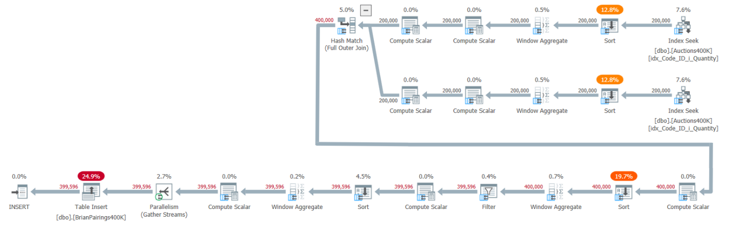 Figure 1: Query plan for Brian’s solution
The top two branches of the plan compute the demand and supply running totals using a batch-mode Window Aggregate operator, each after retrieving the respective entries from the supporting index. Like I explained in earlier articles in the series, since the index already has the rows ordered like the Window Aggregate operators need them to be, you would think explicit Sort operators shouldn’t be required. But SQL Server doesn’t currently support an efficient combination of parallel order-preserving index operation prior to a parallel batch-mode Window Aggregate operator, so as a result, an explicit parallel Sort operator precedes each of the parallel Window Aggregate operators.
The plan uses a batch-mode hash join to handle the full outer join. The plan also uses two additional batch-mode Window Aggregate operators preceded by explicit Sort operators to compute the MIN and LAG window functions.
That’s a pretty efficient plan!
Here are the run times I got for this solution against input sizes ranging from 100K to 400K rows, in seconds:
100K: 0.368
200K: 0.845
300K: 1.255
400K: 1.315
Itzik’s Solution
The next solution for the challenge is one of my attempts at solving it. Here’s the complete solution code:
DROP TABLE IF EXISTS #MyPairings;

WITH C1 AS
(
  SELECT *,
    SUM(Quantity)
      OVER(PARTITION BY Code
           ORDER BY ID
           ROWS UNBOUNDED PRECEDING) AS SumQty
  FROM dbo.Auctions
),
C2 AS
(
  SELECT *,
    SUM(Quantity * CASE Code WHEN 'D' THEN -1 WHEN 'S' THEN 1 END)
      OVER(ORDER BY SumQty, Code
           ROWS UNBOUNDED PRECEDING) AS StockLevel,
    LAG(SumQty, 1, 0.0) OVER(ORDER BY SumQty, Code) AS PrevSumQty,
    MAX(CASE WHEN Code = 'D' THEN ID END)
      OVER(ORDER BY SumQty, Code
           ROWS UNBOUNDED PRECEDING) AS PrevDemandID,
    MAX(CASE WHEN Code = 'S' THEN ID END)
      OVER(ORDER BY SumQty, Code
           ROWS UNBOUNDED PRECEDING) AS PrevSupplyID,
    MIN(CASE WHEN Code = 'D' THEN ID END)
      OVER(ORDER BY SumQty, Code
           ROWS BETWEEN CURRENT ROW AND UNBOUNDED FOLLOWING) AS NextDemandID,
    MIN(CASE WHEN Code = 'S' THEN ID END)
      OVER(ORDER BY SumQty, Code
           ROWS BETWEEN CURRENT ROW AND UNBOUNDED FOLLOWING) AS NextSupplyID
  FROM C1
),
C3 AS
(
  SELECT *,
    CASE Code
      WHEN 'D' THEN ID
      WHEN 'S' THEN
        CASE WHEN StockLevel > 0 THEN NextDemandID ELSE PrevDemandID END
    END AS DemandID,
    CASE Code
      WHEN 'S' THEN ID
      WHEN 'D' THEN
        CASE WHEN StockLevel <= 0 THEN NextSupplyID ELSE PrevSupplyID END
    END AS SupplyID,
    SumQty - PrevSumQty AS TradeQuantity
  FROM C2
)
SELECT DemandID, SupplyID, TradeQuantity
INTO #MyPairings
FROM C3
WHERE TradeQuantity > 0.0
  AND DemandID IS NOT NULL
  AND SupplyID IS NOT NULL;
The CTE C1 queries the Auctions table and uses a window function to compute running total demand and supply quantities, calling the result column SumQty.
The CTE C2 queries C1, and computes a number of attributes using window functions based on SumQty and Code ordering:
- StockLevel: The current stock level after processing each entry. This is computed by assigning a negative sign to demand quantities and a positive sign to supply quantities and summing those quantities up to and including the current entry.
- PrevSumQty: Previous row’s SumQty value.
- PrevDemandID: Last non-NULL demand ID.
- PrevSupplyID: Last non-NULL supply ID.
- NextDemandID: Next non-NULL demand ID.
- NextSupplyID: Next non-NULL supply ID.
Here’s the contents of C2 ordered by SumQty and Code:
ID    Code Quantity  SumQty     StockLevel  PrevSumQty  PrevDemandID PrevSupplyID NextDemandID NextSupplyID
----- ---- --------- ---------- ----------- ----------- ------------ ------------ ------------ ------------
1     D    5.000000   5.000000  -5.000000    0.000000   1            NULL         1            1000
2     D    3.000000   8.000000  -8.000000    5.000000   2            NULL         2            1000
1000  S    8.000000   8.000000   0.000000    8.000000   2            1000         3            1000
2000  S    6.000000  14.000000   6.000000    8.000000   2            2000         3            2000
3     D    8.000000  16.000000  -2.000000   14.000000   3            2000         3            3000
3000  S    2.000000  16.000000   0.000000   16.000000   3            3000         5            3000
5     D    2.000000  18.000000  -2.000000   16.000000   5            3000         5            4000
4000  S    2.000000  18.000000   0.000000   18.000000   5            4000         6            4000
5000  S    4.000000  22.000000   4.000000   18.000000   5            5000         6            5000
6000  S    3.000000  25.000000   7.000000   22.000000   5            6000         6            6000
6     D    8.000000  26.000000  -1.000000   25.000000   6            6000         6            7000
7000  S    2.000000  27.000000   1.000000   26.000000   6            7000         7            7000
7     D    4.000000  30.000000  -3.000000   27.000000   7            7000         7            NULL
8     D    2.000000  32.000000  -5.000000   30.000000   8            7000         8            NULL
The CTE C3 queries C2 and computes the result pairings’ DemandID, SupplyID and TradeQuantity, before removing some superfluous rows.
The result C3.DemandID column is computed like so:
- If the current entry is a demand entry, return DemandID.
- If the current entry is a supply entry and the current stock level is positive, return NextDemandID.
- If the current entry is a supply entry and the current stock level is nonpositive, return PrevDemandID.
The result C3.SupplyID column is computed like so:
- If the current entry is a supply entry, return SupplyID.
- If the current entry is a demand entry and the current stock level is nonpositive, return NextSupplyID.
- If the current entry is a demand entry and the current stock level is positive, return PrevSupplyID.
The result TradeQuantity is computed as the current row’s SumQty minus PrevSumQty.
Here are the contents of the columns relevant to the result from C3:
DemandID    SupplyID    TradeQuantity
----------- ----------- --------------
1           1000        5.000000
2           1000        3.000000
2           1000        0.000000
3           2000        6.000000
3           3000        2.000000
3           3000        0.000000
5           4000        2.000000
5           4000        0.000000
6           5000        4.000000
6           6000        3.000000
6           7000        1.000000
7           7000        1.000000
7           NULL        3.000000
8           NULL        2.000000
What’s left for the outer query to do is to filter out superfluous rows from C3. Those include two cases:
- When the running totals of both kinds are the same, the supply entry has a zero trading quantity. Remember the ordering is based on SumQty and Code, so when the running totals are the same, the demand entry appears before the supply entry.
- Trailing entries of one kind that cannot be matched with entries of the other kind. Such entries are represented by rows in C3 where either the DemandID is NULL or the SupplyID is NULL.
The plan for this solution is shown in Figure 2.
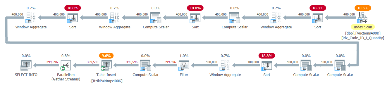 Figure 2: Query plan for Itzik’s solution
The plan applies one pass over the input data and uses four batch-mode Window Aggregate operators to handle the various windowed computations. All Window Aggregate operators are preceded by explicit Sort operators, although only two of those are unavoidable here. The other two have to do with the current implementation of the parallel batch-mode Window Aggregate operator, which cannot rely on a parallel order-preserving input. A simple way to see which Sort operators are due to this reason is to force a serial plan and see which Sort operators disappear. When I force a serial plan with this solution, the first and third Sort operators disappear.
Here are the run times in seconds that I got for this solution:
100K: 0.246
200K: 0.427
300K: 0.616
400K: 0.841>
Ian’s Solution
Ian’s solution is short and efficient. Here’s the complete solution code:
DROP TABLE IF EXISTS #MyPairings;

WITH A AS (
  SELECT *,
    SUM(Quantity) OVER (PARTITION BY Code
                        ORDER BY ID
                        ROWS UNBOUNDED PRECEDING) AS CumulativeQuantity
  FROM dbo.Auctions
), B AS (
  SELECT CumulativeQuantity,
    CumulativeQuantity
      - LAG(CumulativeQuantity, 1, 0)
          OVER (ORDER BY CumulativeQuantity) AS TradeQuantity,
    MAX(CASE WHEN Code = 'D' THEN ID END) AS DemandID,
    MAX(CASE WHEN Code = 'S' THEN ID END) AS SupplyID
  FROM A
  GROUP BY CumulativeQuantity, ID/ID -- bogus grouping to improve row estimate
                                     -- (rows count of Auctions instead of 2 rows)
), C AS (
  -- fill in NULLs with next supply / demand
  -- FIRST_VALUE(ID) IGNORE NULLS OVER ...
  -- would be better, but this will work because the IDs are in CumulativeQuantity order
  SELECT
    MIN(DemandID) OVER (ORDER BY CumulativeQuantity
                        ROWS BETWEEN CURRENT ROW AND UNBOUNDED FOLLOWING) AS DemandID,
    MIN(SupplyID) OVER (ORDER BY CumulativeQuantity
                        ROWS BETWEEN CURRENT ROW AND UNBOUNDED FOLLOWING) AS SupplyID,
    TradeQuantity
  FROM B
)
SELECT DemandID, SupplyID, TradeQuantity
INTO #MyPairings
FROM C
WHERE SupplyID IS NOT NULL  -- trim unfulfilled demands
  AND DemandID IS NOT NULL; -- trim unused supplies
The code in the CTE A queries the Auctions table and computes running total demand and supply quantities using a window function, naming the result column CumulativeQuantity.
The code in the CTE B queries CTE A, and groups the rows by CumulativeQuantity. This grouping achieves a similar effect to Brian’s outer join based on the demand and supply running totals. Ian also added the dummy expression ID/ID to the grouping set to improve the grouping’s original cardinality under estimation. On my machine, this also resulted in using a parallel plan instead of a serial one.
In the SELECT list, the code computes DemandID and SupplyID by retrieving the ID of the respective entry type in the group using the MAX aggregate and a CASE expression. If the ID isn’t present in the group, the result is NULL. The code also computes a result column called TradeQuantity as the current cumulative quantity minus the previous one, retrieved using the LAG window function.
Here are the contents of B:
CumulativeQuantity  TradeQuantity  DemandId  SupplyId
------------------- -------------- --------- ---------
 5.000000           5.000000       1         NULL
 8.000000           3.000000       2         1000
14.000000           6.000000       NULL      2000
16.000000           2.000000       3         3000
18.000000           2.000000       5         4000
22.000000           4.000000       NULL      5000
25.000000           3.000000       NULL      6000
26.000000           1.000000       6         NULL
27.000000           1.000000       NULL      7000
30.000000           3.000000       7         NULL
32.000000           2.000000       8         NULL
The code in the CTE C then queries the CTE B and fills in NULL demand and supply IDs with the next non-NULL demand and supply IDs, using the MIN window function with the frame ROWS BETWEEN CURRENT ROW AND UNBOUNDED FOLLOWING.
Here are the contents of C:
DemandID  SupplyID  TradeQuantity
--------- --------- --------------
1         1000      5.000000
2         1000      3.000000
3         2000      6.000000
3         3000      2.000000
5         4000      2.000000
6         5000      4.000000
6         6000      3.000000
6         7000      1.000000
7         7000      1.000000
7         NULL      3.000000
8         NULL      2.000000
The last step handled by the outer query against C is to remove entries of one kind that cannot be matched with entries of the other kind. That’s done by filtering out rows where either SupplyID is NULL or DemandID is NULL.
The plan for this solution is shown in Figure 3.
 Figure 3: Query plan for Ian’s solution
This plan performs one scan of the input data and uses three parallel batch-mode window aggregate operators to compute the various window functions, all preceded by parallel Sort operators. Two of those are unavoidable as you can verify by forcing a serial plan. The plan also uses a Hash Aggregate operator to handle the grouping and aggregation in the CTE B.
Here are the run times in seconds that I got for this solution:
100K: 0.214
200K: 0.363
300K: 0.546
400K: 0.701
Peter Larsson’s Solution
Peter Larsson’s solution is amazingly short, sweet, and highly efficient. Here’s Peter’s complete solution code:
DROP TABLE IF EXISTS #MyPairings;

WITH cteSource(ID, Code, RunningQuantity)
AS
(
  SELECT ID, Code,
    SUM(Quantity) OVER (PARTITION BY Code ORDER BY ID) AS RunningQuantity
  FROM dbo.Auctions
)
SELECT DemandID, SupplyID, TradeQuantity
INTO #MyPairings
FROM (
       SELECT
         MIN(CASE WHEN Code = 'D' THEN ID ELSE 2147483648 END)
           OVER (ORDER BY RunningQuantity, Code
                 ROWS BETWEEN CURRENT ROW AND UNBOUNDED FOLLOWING) AS DemandID,
         MIN(CASE WHEN Code = 'S' THEN ID ELSE 2147483648 END)
           OVER (ORDER BY RunningQuantity, Code
                 ROWS BETWEEN CURRENT ROW AND UNBOUNDED FOLLOWING) AS SupplyID,
         RunningQuantity
           - COALESCE(LAG(RunningQuantity) OVER (ORDER BY RunningQuantity, Code), 0.0)
             AS TradeQuantity
       FROM cteSource
     ) AS d
WHERE DemandID < 2147483648
  AND SupplyID < 2147483648
  AND TradeQuantity > 0.0;
The CTE cteSource queries the Auctions table and uses a window function to compute running total demand and supply quantities, calling the result column RunningQuantity.
The code defining the derived table d queries cteSource and computes the result pairings’ DemandID, SupplyID, and TradeQuantity, before removing some superfluous rows. All window functions used in those calculations are based on RunningQuantity and Code ordering.
The result column d.DemandID is computed as the minimum demand ID starting with the current or 2147483648 if none is found.
The result column d.SupplyID is computed as the minimum supply ID starting with the current or 2147483648 if none is found.
The result TradeQuantity is computed as the current row’s RunningQuantity value minus the previous row’s RunningQuantity value.
Here are the contents of d:
DemandID  SupplyID    TradeQuantity
--------- ----------- --------------
1         1000        5.000000
2         1000        3.000000
3         1000        0.000000
3         2000        6.000000
3         3000        2.000000
5         3000        0.000000
5         4000        2.000000
6         4000        0.000000
6         5000        4.000000
6         6000        3.000000
6         7000        1.000000
7         7000        1.000000
7         2147483648  3.000000
8         2147483648  2.000000
What’s left for the outer query to do is to filter out superfluous rows from d. Those are cases where the trading quantity is zero, or entries of one kind that cannot be matched with entries from the other kind (with ID 2147483648).
The plan for this solution is shown in Figure 4.
 Figure 4: Query plan for Peter’s solution
Like Ian’s plan, Peter’s plan relies on one scan of the input data and uses three parallel batch-mode window aggregate operators to compute the various window functions, all preceded by parallel Sort operators. Two of those are unavoidable as you can verify by forcing a serial plan. In Peter’s plan, there’s no need for a grouped aggregate operator like in Ian’s plan.
Peter’s critical insight that allowed for such a short solution was the realization that for a relevant entry of either of the kinds, the matching ID of the other kind will always appear later (based on RunningQuantity and Code ordering). After seeing Peter’s solution, it sure felt like I overcomplicated things in mine!
Here are the run times in seconds I got for this solution:
100K: 0.197
200K: 0.412
300K: 0.558
400K: 0.696
Paul White’s Solution
Our last solution was created by Paul White. Here’s the complete solution code:
DROP TABLE IF EXISTS #MyPairings;

CREATE TABLE #MyPairings
(
  DemandID integer NOT NULL,
  SupplyID integer NOT NULL,
  TradeQuantity decimal(19, 6) NOT NULL
);
GO

INSERT #MyPairings
    WITH (TABLOCK)
(
    DemandID,
    SupplyID,
    TradeQuantity
)
SELECT
    Q3.DemandID,
    Q3.SupplyID,
    Q3.TradeQuantity
FROM
(
    SELECT
        Q2.DemandID,
        Q2.SupplyID,
        TradeQuantity =
            -- Interval overlap
            CASE
                WHEN Q2.Code = 'S' THEN
                    CASE
                        WHEN Q2.CumDemand >= Q2.IntEnd THEN Q2.IntLength
                        WHEN Q2.CumDemand > Q2.IntStart THEN Q2.CumDemand - Q2.IntStart
                        ELSE 0.0
                    END
                WHEN Q2.Code = 'D' THEN
                    CASE
                        WHEN Q2.CumSupply >= Q2.IntEnd THEN Q2.IntLength
                        WHEN Q2.CumSupply > Q2.IntStart THEN Q2.CumSupply - Q2.IntStart
                        ELSE 0.0
                    END
            END
    FROM
    (
        SELECT
            Q1.Code,
            Q1.IntStart,
            Q1.IntEnd,
            Q1.IntLength,
            DemandID = MAX(IIF(Q1.Code = 'D', Q1.ID, 0)) OVER (
                    ORDER BY Q1.IntStart, Q1.ID
                    ROWS UNBOUNDED PRECEDING),
            SupplyID = MAX(IIF(Q1.Code = 'S', Q1.ID, 0)) OVER (
                    ORDER BY Q1.IntStart, Q1.ID
                    ROWS UNBOUNDED PRECEDING),
            CumSupply = SUM(IIF(Q1.Code = 'S', Q1.IntLength, 0)) OVER (
                    ORDER BY Q1.IntStart, Q1.ID
                    ROWS UNBOUNDED PRECEDING),
            CumDemand = SUM(IIF(Q1.Code = 'D', Q1.IntLength, 0)) OVER (
                    ORDER BY Q1.IntStart, Q1.ID
                    ROWS UNBOUNDED PRECEDING)
        FROM
        (
            -- Demand intervals
            SELECT
                A.ID,
                A.Code,
                IntStart = SUM(A.Quantity) OVER (
                    ORDER BY A.ID
                    ROWS UNBOUNDED PRECEDING) - A.Quantity,
                IntEnd = SUM(A.Quantity) OVER (
                    ORDER BY A.ID
                    ROWS UNBOUNDED PRECEDING),
                IntLength = A.Quantity
            FROM dbo.Auctions AS A
            WHERE
                A.Code = 'D'

            UNION ALL

            -- Supply intervals
            SELECT
                A.ID,
                A.Code,
                IntStart = SUM(A.Quantity) OVER (
                    ORDER BY A.ID
                    ROWS UNBOUNDED PRECEDING) - A.Quantity,
                IntEnd = SUM(A.Quantity) OVER (
                    ORDER BY A.ID
                    ROWS UNBOUNDED PRECEDING),
                IntLength = A.Quantity
            FROM dbo.Auctions AS A
            WHERE
                A.Code = 'S'
        ) AS Q1
    ) AS Q2
) AS Q3
WHERE
    Q3.TradeQuantity > 0;
The code defining the derived table Q1 uses two separate queries to compute demand and supply intervals based on running totals and unifies the two. For each interval, the code computes its start (IntStart), end (IntEnd), and length (IntLength). Here are the contents of Q1 ordered by IntStart and ID:
ID    Code IntStart   IntEnd     IntLength
----- ---- ---------- ---------- ----------
1     D     0.000000   5.000000  5.000000
1000  S     0.000000   8.000000  8.000000
2     D     5.000000   8.000000  3.000000
3     D     8.000000  16.000000  8.000000
2000  S     8.000000  14.000000  6.000000
3000  S    14.000000  16.000000  2.000000
5     D    16.000000  18.000000  2.000000
4000  S    16.000000  18.000000  2.000000
6     D    18.000000  26.000000  8.000000
5000  S    18.000000  22.000000  4.000000
6000  S    22.000000  25.000000  3.000000
7000  S    25.000000  27.000000  2.000000
7     D    26.000000  30.000000  4.000000
8     D    30.000000  32.000000  2.000000
The code defining the derived table Q2 queries Q1 and computes result columns called DemandID, SupplyID, CumSupply, and CumDemand. All window functions used by this code are based on IntStart and ID ordering and the frame ROWS UNBOUNDED PRECEDING (all rows up to the current).
DemandID is the maximum demand ID up to the current row, or 0 if none exists.
SupplyID is the maximum supply ID up to the current row, or 0 if none exists.
CumSupply is the cumulative supply quantities (supply interval lengths) up to the current row.
CumDemand is the cumulative demand quantities (demand interval lengths) up to the current row.
Here are the contents of Q2:
Code IntStart   IntEnd     IntLength  DemandID  SupplyID  CumSupply  CumDemand
---- ---------- ---------- ---------- --------- --------- ---------- ----------
D     0.000000   5.000000  5.000000   1         0          0.000000   5.000000
S     0.000000   8.000000  8.000000   1         1000       8.000000   5.000000
D     5.000000   8.000000  3.000000   2         1000       8.000000   8.000000
D     8.000000  16.000000  8.000000   3         1000       8.000000  16.000000
S     8.000000  14.000000  6.000000   3         2000      14.000000  16.000000
S    14.000000  16.000000  2.000000   3         3000      16.000000  16.000000
D    16.000000  18.000000  2.000000   5         3000      16.000000  18.000000
S    16.000000  18.000000  2.000000   5         4000      18.000000  18.000000
D    18.000000  26.000000  8.000000   6         4000      18.000000  26.000000
S    18.000000  22.000000  4.000000   6         5000      22.000000  26.000000
S    22.000000  25.000000  3.000000   6         6000      25.000000  26.000000
S    25.000000  27.000000  2.000000   6         7000      27.000000  26.000000
D    26.000000  30.000000  4.000000   7         7000      27.000000  30.000000
D    30.000000  32.000000  2.000000   8         7000      27.000000  32.000000
Q2 already has the final result pairings’ correct DemandID and SupplyID values. The code defining the derived table Q3 queries Q2 and computes the result pairings’ TradeQuantity values as the overlapping segments of the demand and supply intervals. Finally, the outer query against Q3 filters only the relevant pairings where TradeQuantity is positive.
The plan for this solution is shown in Figure 5.
 Figure 5: Query plan for Paul’s solution
The top two branches of the plan are responsible for computing the demand and supply intervals. Both rely on Index Seek operators to get the relevant rows based on index order, and then use parallel batch-mode Window Aggregate operators, preceded by Sort operators that theoretically could have been avoided. The plan concatenates the two inputs, sorts the rows by IntStart and ID to support the subsequent remaining Window Aggregate operator. Only this Sort operator is unavoidable in this plan. The rest of the plan handles the needed scalar computations and the final filter. That’s a very efficient plan!
Here are the run times in seconds I got for this solution:
100K: 0.187
200K: 0.331
300K: 0.369
400K: 0.425
These numbers are pretty impressive!
Performance Comparison
Figure 6 has a performance comparison between all solutions covered in this article.
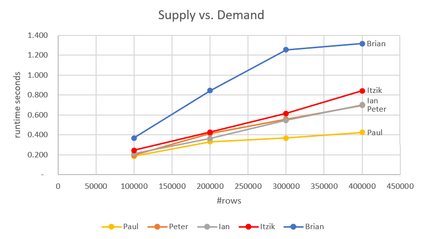 Figure 6: Performance comparison
At this point, we can add the fastest solutions I covered in previous articles. Those are Joe’s and Kamil/Luca/Daniel’s solutions. The complete comparison is shown in Figure 7.
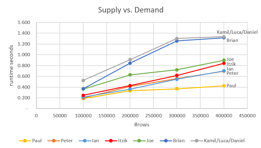 Figure 7: Performance comparison including earlier solutions
These are all impressively fast solutions, with the fastest being Paul’s and Peter’s.
Conclusion
When I originally introduced Peter’s puzzle, I showed a straightforward cursor-based solution that took 11.81 seconds to complete against a 400K-row input. The challenge was to come up with an efficient set-based solution. It’s so inspiring to see all the solutions people sent. I always learn so much from such puzzles both from my own attempts and by analyzing others’ solutions. It’s impressive to see several sub-second solutions, with Paul’s being less than half a second!
It's great to have multiple efficient techniques to handle such a classic need of matching supply with demand. Well done everyone!

Thank you Itzik for the time and effort spent on this article series!
I look forward to send you another quiz :-)
Also a great thank to all who have sent in solutions. There are things to learn from all of you.
This is what I learned from Pauls solutions – split the read part into 2 parallell processes. It shaves of 35% of the execution time!
DROP TABLE IF EXISTS #MyPairings; WITH cteSource(ID, Code, RunningQuantity) AS ( SELECT ID, Code, SUM(Quantity) OVER (ORDER BY ID) AS RunningQuantity FROM dbo.Auctions WHERE Code = 'S' UNION ALL SELECT ID, Code, SUM(Quantity) OVER (ORDER BY ID) AS RunningQuantity FROM dbo.Auctions WHERE Code = 'D' ) SELECT DemandID, SupplyID, TradeQuantity INTO #MyPairings FROM ( SELECT MIN(CASE WHEN Code = 'D' THEN ID ELSE NULL END) OVER (ORDER BY RunningQuantity, Code ROWS BETWEEN CURRENT ROW AND UNBOUNDED FOLLOWING) AS DemandID, MIN(CASE WHEN Code = 'S' THEN ID ELSE NULL END) OVER (ORDER BY RunningQuantity, Code ROWS BETWEEN CURRENT ROW AND UNBOUNDED FOLLOWING) AS SupplyID, RunningQuantity - COALESCE(LAG(RunningQuantity) OVER (ORDER BY RunningQuantity, Code), 0.0) AS TradeQuantity FROM cteSource ) AS d WHERE DemandID IS NOT NULL AND SupplyID IS NOT NULL AND TradeQuantity > 0.0;Hi Peter!
These are the run times in seconds that I get for your revised solution:
100K: 0.175
200K: 0.242
300K: 0.347
400K: 0.427
Slightly faster up to 400k…
I'm surprised by the timings Itzik observed. My timings were different, with my solution being much more competitive.
I tested with a budget laptop as the server. My timings were all much lower duration for 400,000 rows.
When I run Kamil's solution from Part 2, it averages about 0.795 seconds.
When I run Paul's solution from Part 3, it averages about 0.195 seconds. It's extremely fast.
When I run my solution, it averages about 0.0305 seconds. If I add the locking hint used by Paul, my solution averages about 0.235 seconds.
I'm curious what other people observe for timings.
OOPS!
Typo – The 0.0305 should be 0.305.
Hi Brian,
I just went ahead and retested all solutions, and indeed yours is more competitive! I'm not sure what was the issue first time I tested your solution, but I suspect that perhaps there was something else running on my machine at the time, or that I wrote the result to a user table and not a temporary table, or some other factor that affected the test.
At any rate, I just reran all solutions under identical conditions against the 400K-row input three times, and computed the average run times. Here's the result ordered and ranked based on average run time ascending :
Based on this result, the three fastest solutions are (1) Paul's, (2) Peter's revised and (3) yours!
My machine is also a commodity laptop. 5 years old. The specs:
CPU: Intel Core i7-6600U 2.60GHz 2 Cores, 4 Logical Processors
Mem: 16GB RAM
Disk: Crucial MX200 SSD
OS: Windows 11 Pro
SQL: SQL Server 2019 Enterprise
Again, all of the solutions in this article + Kamil's + Joe's are very impressive, with Paul's being the fastest. Thanks much for checking this and for the catch!
Hi Itzik,
Thanks for rechecking the numbers! It's good to know I was not going crazy with my findings!
I agree about all of the solutions. There's plenty to learn from all of them, and from your articles exploring them.
Brian
This has been a great challenge, I have learned a great deal from other solutions (still have material to go through :-)).
Congrats to the winners and thanks Itzik for taking time to write about the problem in such way that encourages hands-on participation and a bit of competition.
I look forward to the next challenge!
Thanks Brian and Kamil!
Great series.
It seems strange you would include the INSERT into a temp table. Paul gets a boost simply by adding a TABLOCK but no-one else does??
I would think the fastest way to test this is to actually SELECT back to the client, then just discard the results (for example SSMS has a Discard Results option).
Thanks Charlie!
Every test has its flaws. Returning the result to the client and discarding results still involves the time it takes to send the results through the network. When Peter sent me the challenge originally, before we even thought of sharing it with everyone, he actually needed to write the result into a table. It was a regular table and not a temporary one, but we decided to simplify things a bit for the puzzle. The instruction was to write the result into a temporary table with no further info. This means that it was fair game for anyone to decide how to write to the temp table; be it INSERT SELECT, with or without the TABLOCK hint, or SELECT INTO. I basically ran the code that people sent me.
Paul got a performance boost with his TABLOCK hint simply because he was the only one who included it in his solution. :) A couple of us used a SELECT INTO and not INSERT SELECT.
Thank you for the problem and the solutions! They were very educational.
Have you considered another round to update these solutions to support sorting by something other than the ID? Matching the smallest demand quantities to the largest supply quantities for instance. It would be interesting to see the performance implications of different techniques used for achieving the sort.
Thanks Brian!
There are all sorts of variations to the original problem that could indeed be very interesting to test.
Great Solution @Brian Walker.
i have tested your solotion againg and aging and found out that every thing is perfect the way it should be.
but i have a question is this applicable for ID when data type is uniqueidentifier