
T-SQL bugs, pitfalls, and best practices – window functions
This article is the fourth installment in a series about T-SQL bugs, pitfalls and best practices. Previously I covered determinism, subqueries and joins. The focus of this month’s article is bugs, pitfalls and best practices related to window functions. Thanks Erland Sommarskog, Aaron Bertrand, Alejandro Mesa, Umachandar Jayachandran (UC), Fabiano Neves Amorim, Milos Radivojevic, Simon Sabin, Adam Machanic, Thomas Grohser, Chan Ming Man and Paul White for offering your ideas!
In my examples I’ll use a sample database called TSQLV5. You can find the script that creates and populates this database here, and its ER diagram here.
There are two common pitfalls involving window functions, both of which are the result of counterintuitive implicit defaults that are imposed by the SQL standard. One pitfall has to do with calculations of running totals where you get a window frame with the implicit RANGE option. Another pitfall is somewhat related, but has more severe consequences, involving an implicit frame definition for the FIRST_VALUE and LAST_VALUE functions.
Window frame with implicit RANGE option
Our first pitfall involves the computation of running totals using an aggregate window function, where you do explicitly specify the window order clause, but you do not explicitly specify the window frame unit (ROWS or RANGE) and its related window frame extent, e.g., ROWS UNBOUNDED PRECEDING. The implicit default is counterintuitive and its consequences could be surprising and painful.
To demonstrate this pitfall, I’ll use a table called Transactions holding two million bank account transactions with credits (positive values) and debits (negative values). Run the following code to create the Transactions table and populate it with sample data:
  SET NOCOUNT ON;

  USE TSQLV5; -- http://tsql.solidq.com/SampleDatabases/TSQLV5.zip

  DROP TABLE IF EXISTS dbo.Transactions;

  CREATE TABLE dbo.Transactions
  (
    actid  INT   NOT NULL,
    tranid INT   NOT NULL,
    val    MONEY NOT NULL,
    CONSTRAINT PK_Transactions PRIMARY KEY(actid, tranid) -- creates POC index
  );

  DECLARE
    @num_partitions     AS INT = 100,
    @rows_per_partition AS INT = 20000;

  INSERT INTO dbo.Transactions WITH (TABLOCK) (actid, tranid, val)
    SELECT NP.n, RPP.n,
      (ABS(CHECKSUM(NEWID())%2)*2-1) * (1 + ABS(CHECKSUM(NEWID())%5))
    FROM dbo.GetNums(1, @num_partitions) AS NP
      CROSS JOIN dbo.GetNums(1, @rows_per_partition) AS RPP;
Our pitfall has both a logical side to it with a potential logical bug as well as a performance side with a performance penalty. The performance penalty is relevant only when the window function is optimized with row-mode processing operators. SQL Server 2016 introduces the batch-mode Window Aggregate operator, which removes the performance penalty part of the pitfall, but prior to SQL Server 2019 this operator is used only if you have a columnstore index present on the data. SQL Server 2019 introduces batch mode on rowstore support, so you can get batch-mode processing even if there’s no columnstore indexes present on the data. To demonstrate the performance penalty with the row-mode processing, if you’re running the code samples in this article on SQL Server 2019 or later, or on Azure SQL Database, use the following code to set the database compatibility level to 140 so as not to enable batch-mode on row store yet:
ALTER DATABASE TSQLV5 SET COMPATIBILITY_LEVEL = 140;Use the following code to turn on time and I/O statistics in the session:
SET STATISTICS TIME, IO ON;To avoid waiting for two million rows to be printed in SSMS, I suggest running the code samples in this section with the Discard results after execution option turned on (go to Query Options, Results, Grid, and check Discard results after execution).
Before we get to the pitfall, consider the following query (call it Query 1) which computes the bank account balance after each transaction by applying a running total using a window aggregate function with an explicit frame specification:
  SELECT actid, tranid, val,
    SUM(val) OVER( PARTITION BY actid
                   ORDER BY tranid
                   ROWS UNBOUNDED PRECEDING ) AS balance
  FROM dbo.Transactions;
The plan for this query, using row-mode processing, is shown in Figure 1.
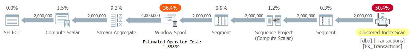 Figure 1: Plan for Query 1, row-mode processing
The plan pulls the data preordered from the table’s clustered index. Then it uses the Segment and Sequence Project operators to compute row numbers to figure out which rows belong to the current row’s frame. Then it uses the Segment, Window Spool and Stream Aggregate operators to compute the window aggregate function. The Window Spool operator is used to spool the frame rows that then need to be aggregated. Without any special optimization, the plan would have had to write per row all of its applicable frame rows to the spool, and then aggregate them. This would have resulted in quadratic, or N2, complexity. The good news is that when the frame starts with UNBOUNDED PRECEDING, SQL Server identifies the case as a fast track case, in which it simply takes the previous row’s running total and adds the current row’s value to compute the current row’s running total, resulting in linear scaling. In this fast track mode, the plan writes only two rows to the spool per input row—one with the aggregate, and one with the detail.
The Window Spool can be physically implemented in one of two ways. Either as a fast in-memory spool that was especially designed for window functions, or as a slow on-disk spool, which is essentially a temporary table in tempdb. If the number of rows that need to be written to the spool per underlying row could exceed 10,000, or if SQL Server cannot predict the number, it will use the slower on-disk spool. In our query plan, we have exactly two rows written to the spool per underlying row, so SQL Server uses the in-memory spool. Unfortunately, there’s no way to tell from the plan what kind of spool you’re getting. There are two ways to figure this out. One is to use an extended event called window_spool_ondisk_warning. Another option is to enable STATISTICS IO, and to check the number of logical reads reported for a table called Worktable. A greater than zero number means you got the on-disk spool. Zero means you got the in-memory spool. Here’s the I/O statistics for our query:
As you can see, we got the in-memory spool used. That’s generally the case when you use the ROWS window frame unit with UNBOUNDED PRECEDING as the first delimiter.
Here are the time statistics for our query:
It took this query about 4.5 seconds to complete on my machine with results discarded.
Now for the catch. If you use the RANGE option instead of ROWS, with the same delimiters, there may be a subtle difference in meaning, but a big difference in performance in row mode. The difference in meaning is only relevant if you don’t have total ordering, i.e., if you’re ordering by something that isn’t unique. The ROWS UNBOUNDED PRECEDING option stops with the current row, so in case of ties, the calculation is nondeterministic. Conversely, the RANGE UNBOUNDED PRECEDING option looks ahead of the current row, and includes ties if present. It uses similar logic to the TOP WITH TIES option. When you do have total ordering, i.e., you’re ordering by something unique, there are no ties to include, and therefore ROWS and RANGE become logically equivalent in such a case. The problem is that when you use RANGE, SQL Server always uses the on-disk spool under row-mode processing since when processing a given row it can’t predict how many more rows will be included. This can have a severe performance penalty.
Consider the following query (call it Query 2), which is the same as Query 1, only using the RANGE option instead of ROWS:
  SELECT actid, tranid, val,
    SUM(val) OVER( PARTITION BY actid
                   ORDER BY tranid
                   RANGE UNBOUNDED PRECEDING ) AS balance
  FROM dbo.Transactions;
The plan for this query is shown in Figure 2.
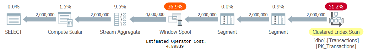 Figure 2: Plan for Query 2, row-mode processing
Query 2 is logically equivalent to Query 1 because we have total order; however, since it uses RANGE, it gets optimized with the on-disk spool. Observe that in the plan for Query 2 the Window Spool looks the same as in the plan for Query 1, and the estimated costs are the same.
Here are the time and I/O statistics for the execution of Query 2:
Table 'Worktable' logical reads: 12044701. Table 'Transactions' logical reads: 6208.
Notice the large number of logical reads against Worktable, indicating that you got the on-disk spool. The run time is more than four times longer than for Query 1.
If you’re thinking that if that’s the case, you’ll simply avoid using the RANGE option, unless you really need to include ties, that’s good thinking. The problem is that if you use a window function that supports a frame (aggregates, FIRST_VALUE, LAST_VALUE) with an explicit window order clause, but no mention of the window frame unit and its associated extent, you’re getting RANGE UNBOUNDED PRECEDING by default. This default is dictated by the SQL standard, and the standard chose it because it generally prefers more deterministic options as defaults. The following query (call it Query 3) is an example that falls into this trap:
  SELECT actid, tranid, val,
    SUM(val) OVER( PARTITION BY actid
                   ORDER BY tranid ) AS balance
  FROM dbo.Transactions;
Often people write like this assuming they’re getting ROWS UNBOUNDED PRECEDING by default, not realizing that they’re actually getting RANGE UNBOUNDED PRECEDING. The thing is that since the function uses total order, you do get the same result like with ROWS, so you can’t tell that there’s a problem from the result. But the performance numbers that you will get are like for Query 2. I see people falling into this trap all the time.
The best practice to avoid this problem is in cases where you use a window function with a frame, be explicit about the window frame unit and its extent, and generally prefer ROWS. Reserve the use of RANGE only to cases where ordering isn’t unique and you need to include ties.
Consider the following query illustrating a case when there is a conceptual difference between ROWS and RANGE:
  SELECT orderdate, orderid, val,
    SUM(val) OVER( ORDER BY orderdate ROWS UNBOUNDED PRECEDING ) AS sumrows,
    SUM(val) OVER( ORDER BY orderdate RANGE UNBOUNDED PRECEDING ) AS sumrange
  FROM Sales.OrderValues
  ORDER BY orderdate;
This query generates the following output:
  orderdate  orderid  val      sumrows  sumrange
  ---------- -------- -------- -------- ---------
  2017-07-04 10248    440.00   440.00   440.00
  2017-07-05 10249    1863.40  2303.40  2303.40
  2017-07-08 10250    1552.60  3856.00  4510.06
  2017-07-08 10251    654.06   4510.06  4510.06
  2017-07-09 10252    3597.90  8107.96  8107.96
  ...
Observe the difference in the results for the rows where the same order date appears more than once, as is the case for July 8th, 2017. Notice how the ROWS option doesn’t include ties and hence is nondeterministic, and how the RANGE option does include ties, and hence is always deterministic.
It’s questionable though if in practice you have cases where you order by something that isn’t unique, and you really need inclusion of ties to make the calculation deterministic. What’s probably much more common in practice is to do one of two things. One is to break ties by adding something to the window ordering to makes it unique and this way result in a deterministic calculation, like so:
  SELECT orderdate, orderid, val,
    SUM(val) OVER( ORDER BY orderdate, orderid ROWS UNBOUNDED PRECEDING ) AS runningsum
  FROM Sales.OrderValues
  ORDER BY orderdate;
This query generates the following output:
  orderdate  orderid  val       runningsum
  ---------- -------- --------- -----------
  2017-07-04 10248    440.00    440.00
  2017-07-05 10249    1863.40   2303.40
  2017-07-08 10250    1552.60   3856.00
  2017-07-08 10251    654.06    4510.06
  2017-07-09 10252    3597.90   8107.96
  ...
Another option is to apply preliminary grouping, in our case, by order date, like so:
  SELECT orderdate, SUM(val) AS daytotal,
    SUM(SUM(val)) OVER( ORDER BY orderdate ROWS UNBOUNDED PRECEDING ) AS runningsum
  FROM Sales.OrderValues
  GROUP BY orderdate
  ORDER BY orderdate;
This query generates the following output where each order date appears only once:
  orderdate  daytotal  runningsum
  ---------- --------- -----------
  2017-07-04 440.00    440.00
  2017-07-05 1863.40   2303.40
  2017-07-08 2206.66   4510.06
  2017-07-09 3597.90   8107.96
  ...
At any rate, make sure to remember the best practice here!
The good news is that if you’re running on SQL Server 2016 or later and have a columnstore index present on the data (even if it’s a fake filtered columnstore index), or if you're running on SQL Server 2019 or later, or on Azure SQL Database, irrespective of the presence of columnstore indexes, all three aforementioned queries get optimized with the batch-mode Window Aggregate operator. With this operator, many of the row-mode processing inefficiencies are eliminated. This operator doesn’t use a spool at all, so there’s no issue of in-memory versus on-disk spool. It uses more sophisticated processing where it can apply multiple parallel passes over the window of rows in memory for both ROWS and RANGE.
To demonstrate using the batch-mode optimization, make sure your database compatibility level is set to 150 or higher:
ALTER DATABASE TSQLV5 SET COMPATIBILITY_LEVEL = 150;Run Query 1 again:
  SELECT actid, tranid, val,
    SUM(val) OVER( PARTITION BY actid
                   ORDER BY tranid
                   ROWS UNBOUNDED PRECEDING ) AS balance
  FROM dbo.Transactions;
The plan for this query is shown in Figure 3.
 Figure 3: Plan for Query 1, batch-mode processing
Here are the performance statistics that I got for this query:
Table 'Transactions' logical reads: 6208.
The run time dropped to 1 second!
Run Query 2 with the explicit RANGE option again:
  SELECT actid, tranid, val,
    SUM(val) OVER( PARTITION BY actid
                   ORDER BY tranid
                   RANGE UNBOUNDED PRECEDING ) AS balance
  FROM dbo.Transactions;
The plan for this query is shown in Figure 4.
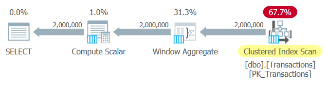 Figure 2: Plan for Query 2, batch-mode processing
Here are the performance statistics that I got for this query:
Table 'Transactions' logical reads: 6208.
The performance is the same as for Query 1.
Run Query 3 again, with the implicit RANGE option:
  SELECT actid, tranid, val,
    SUM(val) OVER( PARTITION BY actid
                   ORDER BY tranid ) AS balance
  FROM dbo.Transactions;
The plan and the performance numbers are of course the same as for Query 2.
When you’re done, run the following code to turn off performance statistics:
SET STATISTICS TIME, IO OFF;Also, don’t forget to turn off the Discard results after execution option in SSMS.
Implicit frame with FIRST_VALUE and LAST_VALUE
The FIRST_VALUE and LAST_VALUE functions are offset window functions that return an expression from the first or last row in the window frame, respectively. The tricky part about them is that often when people use them for the first time, they don’t realize that they support a frame, rather think that they apply to the whole partition.
Consider the following attempt to return order info, plus the values of the customer's first and last orders:
  SELECT custid, orderdate, orderid, val,
    FIRST_VALUE(val) OVER( PARTITION BY custid
                           ORDER BY orderdate, orderid ) AS firstval,
    LAST_VALUE(val) OVER( PARTITION BY custid
                           ORDER BY orderdate, orderid ) AS lastval
  FROM Sales.OrderValues
  ORDER BY custid, orderdate, orderid;
If you incorrectly believe that these functions operate on the entire window partition, which is the belief of many people who use these functions for the first time, you naturally expect FIRST_VALUE to return the order value of the customer’s first order, and LAST_VALUE to return the order value of the customer’s last order. In practice, though, these functions support a frame. As a reminder, with functions that support a frame, when you specify the window order clause but not the window frame unit and its associated extent, you get RANGE UNBOUNDED PRECEDING by default. With the FIRST_VALUE function, you will get the expected result, but if your query gets optimized with row-mode operators, you will pay the penalty of using the on-disk spool. With the LAST_VALUE function it’s even worse. Not only that you will pay the penalty of the on-disk spool, but instead of getting the value from the last row in the partition, you will get the value from the current row!
Here’s the output of the above query:
  custid  orderdate  orderid  val        firstval   lastval
  ------- ---------- -------- ---------- ---------- ----------
  1       2018-08-25 10643    814.50     814.50     814.50
  1       2018-10-03 10692    878.00     814.50     878.00
  1       2018-10-13 10702    330.00     814.50     330.00
  1       2019-01-15 10835    845.80     814.50     845.80
  1       2019-03-16 10952    471.20     814.50     471.20
  1       2019-04-09 11011    933.50     814.50     933.50
  2       2017-09-18 10308    88.80      88.80      88.80
  2       2018-08-08 10625    479.75     88.80      479.75
  2       2018-11-28 10759    320.00     88.80      320.00
  2       2019-03-04 10926    514.40     88.80      514.40
  3       2017-11-27 10365    403.20     403.20     403.20
  3       2018-04-15 10507    749.06     403.20     749.06
  3       2018-05-13 10535    1940.85    403.20     1940.85
  3       2018-06-19 10573    2082.00    403.20     2082.00
  3       2018-09-22 10677    813.37     403.20     813.37
  3       2018-09-25 10682    375.50     403.20     375.50
  3       2019-01-28 10856    660.00     403.20     660.00
  ...
Often when people see such output for the first time, they think that SQL Server has a bug. But of course, it doesn’t; it’s simply the SQL standard’s default. There’s a bug in the query. Realizing that there’s a frame involved, you want to be explicit about the frame specification, and use the minimum frame that captures the row that you’re after. Also, make sure that you use the ROWS unit. So, to get the first row in the partition, use the FIRST_VALUE function with the frame ROWS BETWEEN UNBOUNDED PRECEDING AND CURRENT ROW. To get the last row in the partition, use the LAST_VALUE function with the frame ROWS BETWEEN CURRENT ROW AND UNBOUNDED FOLLOWING.
Here’s our revised query with the bug fixed:
  SELECT custid, orderdate, orderid, val,
    FIRST_VALUE(val) OVER( PARTITION BY custid
                           ORDER BY orderdate, orderid
                           ROWS BETWEEN UNBOUNDED PRECEDING AND CURRENT ROW ) AS firstval,
    LAST_VALUE(val) OVER( PARTITION BY custid
                          ORDER BY orderdate, orderid
                          ROWS BETWEEN CURRENT ROW AND UNBOUNDED FOLLOWING ) AS lastval
  FROM Sales.OrderValues
  ORDER BY custid, orderdate, orderid;
This time you get the correct result:
  custid  orderdate  orderid  val        firstval   lastval
  ------- ---------- -------- ---------- ---------- ----------
  1       2018-08-25 10643    814.50     814.50     933.50
  1       2018-10-03 10692    878.00     814.50     933.50
  1       2018-10-13 10702    330.00     814.50     933.50
  1       2019-01-15 10835    845.80     814.50     933.50
  1       2019-03-16 10952    471.20     814.50     933.50
  1       2019-04-09 11011    933.50     814.50     933.50
  2       2017-09-18 10308    88.80      88.80      514.40
  2       2018-08-08 10625    479.75     88.80      514.40
  2       2018-11-28 10759    320.00     88.80      514.40
  2       2019-03-04 10926    514.40     88.80      514.40
  3       2017-11-27 10365    403.20     403.20     660.00
  3       2018-04-15 10507    749.06     403.20     660.00
  3       2018-05-13 10535    1940.85    403.20     660.00
  3       2018-06-19 10573    2082.00    403.20     660.00
  3       2018-09-22 10677    813.37     403.20     660.00
  3       2018-09-25 10682    375.50     403.20     660.00
  3       2019-01-28 10856    660.00     403.20     660.00
  ...
One wonders what was the motivation for the standard to even support a frame with these functions. If you think about it, you will mostly use them to get something from the first or last rows in the partition. If you need the value from, say, two rows before the current, instead of using FIRST_VALUE with a frame that starts with 2 PRECEDING, isn’t it much easier to use LAG with an explicit offset of 2, like so:
  SELECT custid, orderdate, orderid, val,
    LAG(val, 2) OVER( PARTITION BY custid
                      ORDER BY orderdate, orderid ) AS prevtwoval
  FROM Sales.OrderValues
  ORDER BY custid, orderdate, orderid;
This query generates the following output:
  custid  orderdate  orderid  val        prevtwoval
  ------- ---------- -------- ---------- -----------
  1       2018-08-25 10643    814.50     NULL
  1       2018-10-03 10692    878.00     NULL
  1       2018-10-13 10702    330.00     814.50
  1       2019-01-15 10835    845.80     878.00
  1       2019-03-16 10952    471.20     330.00
  1       2019-04-09 11011    933.50     845.80
  2       2017-09-18 10308    88.80      NULL
  2       2018-08-08 10625    479.75     NULL
  2       2018-11-28 10759    320.00     88.80
  2       2019-03-04 10926    514.40     479.75
  3       2017-11-27 10365    403.20     NULL
  3       2018-04-15 10507    749.06     NULL
  3       2018-05-13 10535    1940.85    403.20
  3       2018-06-19 10573    2082.00    749.06
  3       2018-09-22 10677    813.37     1940.85
  3       2018-09-25 10682    375.50     2082.00
  3       2019-01-28 10856    660.00     813.37
  ...
Apparently, there is a semantic difference between the above use of the LAG function and FIRST_VALUE with a frame that starts with 2 PRECEDING. With the former, if a row doesn’t exist in the desired offset, you get a NULL by default. With the latter, you still get the value from the first row that is present, i.e., the value from the first row in the partition. Consider the following query:
  SELECT custid, orderdate, orderid, val,
    FIRST_VALUE(val) OVER( PARTITION BY custid
                           ORDER BY orderdate, orderid
                           ROWS BETWEEN 2 PRECEDING AND CURRENT ROW ) AS prevtwoval
  FROM Sales.OrderValues
  ORDER BY custid, orderdate, orderid;
This query generates the following output:
  custid  orderdate  orderid  val        prevtwoval
  ------- ---------- -------- ---------- -----------
  1       2018-08-25 10643    814.50     814.50
  1       2018-10-03 10692    878.00     814.50
  1       2018-10-13 10702    330.00     814.50
  1       2019-01-15 10835    845.80     878.00
  1       2019-03-16 10952    471.20     330.00
  1       2019-04-09 11011    933.50     845.80
  2       2017-09-18 10308    88.80      88.80
  2       2018-08-08 10625    479.75     88.80
  2       2018-11-28 10759    320.00     88.80
  2       2019-03-04 10926    514.40     479.75
  3       2017-11-27 10365    403.20     403.20
  3       2018-04-15 10507    749.06     403.20
  3       2018-05-13 10535    1940.85    403.20
  3       2018-06-19 10573    2082.00    749.06
  3       2018-09-22 10677    813.37     1940.85
  3       2018-09-25 10682    375.50     2082.00
  3       2019-01-28 10856    660.00     813.37
  ...
Observe that this time that are no NULLs in the output. So there is some value in supporting a frame with FIRST_VALUE and LAST_VALUE. Just make sure that you remember the best practice to always be explicit about the frame specification with these functions, and to use the ROWS option with the minimal frame that contains the row that you’re after.
Conclusion
This article focused on bugs, pitfalls and best practices related to window functions. Remember that both window aggregate functions and the FIRST_VALUE and LAST_VALUE window offset functions support a frame, and that if you specify the window order clause but you don’t specify the window frame unit and its associated extent, you’re getting RANGE UNBOUNDED PRECEDING by default. This incurs a performance penalty when the query gets optimized with row-mode operators. With the LAST_VALUE function this results in getting the values from the current row instead of the last row in the partition. Remember to be explicit about the frame and to generally prefer the ROWS option to RANGE. It’s great to see the performance improvements with the batch-mode Window Aggregate operator. When it’s applicable, at least the performance pitfall is eliminated.