The Adaptive Join Threshold

First introduced in SQL Server 2017 Enterprise Edition, an adaptive join enables a runtime transition from a batch mode hash join to a row mode correlated nested loops indexed join (apply) at runtime. For brevity, I’ll refer to a “correlated nested loops indexed join” as an apply throughout the rest of this article. If you need a refresher on the difference between nested loops and apply, please see my previous article.

Whether an adaptive join transitions from a hash join to apply at runtime depends on a value labelled Adaptive Threshold Rows on the Adaptive Join execution plan operator. This article shows how an adaptive join works, includes details of the threshold calculation, and covers the implications of some of the design choices made.

Introduction

One thing I want you to bear in mind throughout this piece is an adaptive join always starts executing as a batch mode hash join. This is true even if the execution plan indicates the adaptive join expects to run as a row mode apply.

Like any hash join, an adaptive join reads all rows available on its build input and copies the required data into a hash table. The batch mode flavour of hash join stores these rows in an optimized format, and partitions them using one or more hash functions. Once the build input has been consumed, the hash table is fully populated and partitioned, ready for the hash join to start checking probe-side rows for matches.

This is the point where an adaptive join makes the decision to proceed with the batch mode hash join or to transition to a row mode apply. If the number of rows in the hash table is less than the threshold value, the join switches to an apply; otherwise, the join continues as a hash join by starting to read rows from the probe input.

If a transition to an apply join occurs, the execution plan doesn’t reread the rows used to populate the hash table to drive the apply operation. Instead, an internal component known as an adaptive buffer reader expands the rows already stored in the hash table and makes them available on-demand to the outer input of the apply operator. There’s a cost associated with the adaptive buffer reader, but it’s much lower than the cost of completely rewinding the build input.

Choosing an Adaptive Join

Query optimization involves one or more stages of logical exploration and physical implementation of alternatives. At each stage, when the optimizer explores the physical options for a logical join, it might consider both batch mode hash join and row mode apply alternatives.

If one of those physical join options forms part of the cheapest solution found during the current stage—and the other type of join can deliver the same required logical properties—the optimizer marks the logical join group as potentially suitable for an adaptive join. If not, consideration of an adaptive join ends here (and no adaptive join extended event is fired).

The normal operation of the optimizer means the cheapest solution found will only include one of the physical join options—either hash or apply, whichever had the lowest estimated cost. The next thing the optimizer does is build and cost a fresh implementation of the type of join that wasn’t chosen as cheapest.

Since the current optimization phase has already ended with a cheapest solution found, a special single-group exploration and implementation round is performed for the adaptive join. Finally, the optimizer calculates the adaptive threshold.

If any of the preceding work is unsuccessful, the extended event adaptive_join_skipped is fired with a reason.

If the adaptive join processing is successful, a Concat operator is added to the internal plan above the hash and apply alternatives with the adaptive buffer reader and any required batch/row mode adapters. Remember, only one of the join alternatives will execute at runtime, depending on the number of rows actually encountered compared with the adaptive threshold.

The Concat operator and individual hash/apply alternatives aren’t normally shown in the final execution plan. We’re instead presented with a single Adaptive Join operator. This is a just a presentation decision—the Concat and joins are still present in the code run by the SQL Server execution engine. You can find more details about this in the Appendix and Related Reading sections of this article.

The Adaptive Threshold

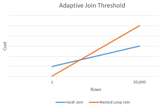
An apply is generally cheaper than a hash join for a smaller number of driving rows. The hash join has an extra startup cost to build its hash table but a lower per-row cost when it starts probing for matches.

There's generally a point where the estimated cost of an apply and hash join will be equal. This idea was nicely illustrated by Joe Sack in his article, Introducing Batch Mode Adaptive Joins:

Calculating the Threshold

At this point, the optimizer has a single estimate for the number of rows entering the build input of the hash join and apply alternatives. It also has the estimated cost of the hash and apply operators as a whole.

This gives us a single point on the extreme right edge of the orange and blue lines in the diagram above. The optimizer needs another point of reference for each join type so it can “draw the lines” and find the intersection (it doesn’t literally draw lines, but you get the idea).

To find a second point for the lines, the optimizer asks the two joins to produce a new cost estimate based on a different (and hypothetical) input cardinality. If the first cardinality estimate was more than 100 rows, it asks the joins to estimate new costs for one row. If the original cardinality was less than or equal to 100 rows, the second point is based on an input cardinality of 10,000 rows (so there’s a decent enough range to extrapolate).

In any case, the result is two different costs and row counts for each join type, allowing the lines to be “drawn.”

The Intersection Formula

Finding the intersection of two lines based on two points for each line is a problem with several well-known solutions. SQL Server uses one based on determinants as described on Wikipedia:

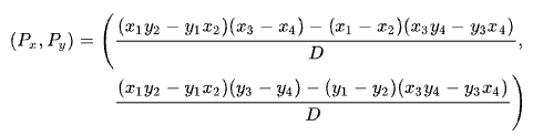
where:

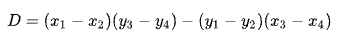
The first line is defined by the points (x₁, y₁) and (x₂, y₂). The second line is given by the points (x₃, y₃) and (x₄, y₄). The intersection is at (P_x, P_y).

Our scheme has the number of rows on the x-axis and the estimated cost on the y-axis. We’re interested in the number of rows where the lines intersect. This is given by the formula for P_x. If we wanted to know the estimated cost at the intersection, it would be P_y.

For P_x rows, the estimated costs of the apply and hash join solutions would be equal. This is the adaptive threshold we need.

A Worked Example

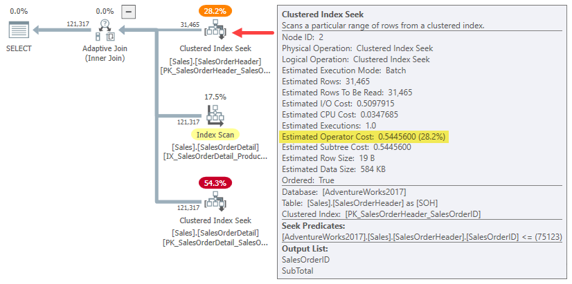
Here’s an example using the AdventureWorks2017 sample database and the following indexing trick by Itzik Ben-Gan to get unconditional consideration of batch mode execution:

-- Itzik's trick
CREATE NONCLUSTERED COLUMNSTORE INDEX BatchMode
ON Sales.SalesOrderHeader (SalesOrderID)
WHERE SalesOrderID = -1
AND SalesOrderID = -2;

-- Test query
SELECT SOH.SubTotal
FROM Sales.SalesOrderHeader AS SOH
JOIN Sales.SalesOrderDetail AS SOD
    ON SOD.SalesOrderID = SOH.SalesOrderID
WHERE SOH.SalesOrderID <= 75123;

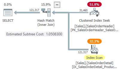
The execution plan shows an adaptive join with a threshold of 1502.07 rows:

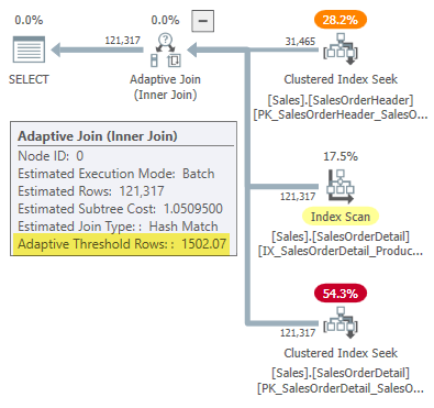
The estimated number of rows driving the adaptive join is 31,465.

Join Costs

In this simplified case, we can find estimated subtree costs for the hash and apply join alternatives using hints:

-- Hash
SELECT SOH.SubTotal
FROM Sales.SalesOrderHeader AS SOH
JOIN Sales.SalesOrderDetail AS SOD
    ON SOD.SalesOrderID = SOH.SalesOrderID
WHERE SOH.SalesOrderID <= 75123
OPTION (HASH JOIN, MAXDOP 1);

-- Apply
SELECT SOH.SubTotal
FROM Sales.SalesOrderHeader AS SOH
JOIN Sales.SalesOrderDetail AS SOD
    ON SOD.SalesOrderID = SOH.SalesOrderID
WHERE SOH.SalesOrderID <= 75123
OPTION (LOOP JOIN, MAXDOP 1);

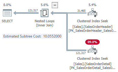
This gives us one point on the line for each join type:

• 31,465 rows
  • Hash cost 1.05083
  • Apply cost 10.0552

The Second Point on the Line

Since the estimated number of rows is more than 100, the second reference points come from special internal estimates based on one join input row. Unfortunately, there’s no easy way to obtain the exact cost numbers for this internal calculation (I’ll talk more about this shortly).

For now, I’ll just show you the cost numbers (using the full internal precision rather than the six significant figures presented in execution plans):

• One row (internal calculation)
  • Hash cost 0.999027422729
  • Apply cost 0.547927305023
• 31,465 rows
  • Hash cost 1.05082787359
  • Apply cost 10.0552890166

As expected, the apply join is cheaper than the hash for a small input cardinality but much more expensive for the expected cardinality of 31,465 rows.

The Intersection Calculation

Plugging these cardinality and cost numbers into the line intersection formula gives you the following:

-- Hash points (x = cardinality; y = cost)

DECLARE 
    @x1 float = 1, 
    @y1 float = 0.999027422729,
    @x2 float = 31465, 
    @y2 float = 1.05082787359;

-- Apply points (x = cardinality; y = cost)

DECLARE
    @x3 float = 1, 
    @y3 float = 0.547927305023,
    @x4 float = 31465, 
    @y4 float = 10.0552890166;

-- Formula:

SELECT Threshold =
    (
        (@x1 * @y2 - @y1 * @x2) * (@x3 - @x4) - 
        (@x1 - @x2) * (@x3 * @y4 - @y3 * @x4)
    )
    /
    (
        (@x1 - @x2) * (@y3 - @y4) - 
        (@y1 - @y2) * (@x3 - @x4)
    );

-- Returns 1502.06521571273

Rounded to six significant figures, this result matches the 1502.07 rows shown in the adaptive join execution plan:

Defect or Design?

Remember, SQL Server needs four points to “draw” the row count versus cost lines to find the adaptive join threshold. In the present case, this means finding cost estimations for the one-row and 31,465-row cardinalities for both apply and hash join implementations.

The optimizer calls a routine named sqllang!CuNewJoinEstimate to calculate these four costs for an adaptive join. Sadly, there are no trace flags or extended events to provide a handy overview of this activity. The normal trace flags used to investigate optimizer behaviour and display costs don’t function here (see the Appendix if you’re interested in more details).

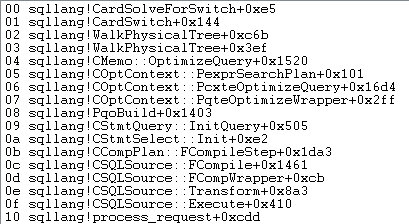
The only way to obtain the one-row cost estimates is to attach a debugger and set a breakpoint after the fourth call to CuNewJoinEstimate in the code for sqllang!CardSolveForSwitch. I used WinDbg to obtain this call stack on SQL Server 2019 CU12:

At this point in the code, double-precision floating points costs are stored in four memory locations pointed to by addresses at rsp+b0, rsp+d0, rsp+30, and rsp+28 (where rsp is a CPU register and offsets are in hexadecimal):

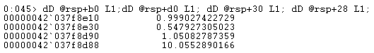
The operator subtree cost numbers shown match those used in the adaptive join threshold calculation formula.

About Those One-Row Cost Estimates

You may have noticed the estimated subtree costs for the one-row joins seem quite high for the amount of work involved in joining one row:

• One row
  • Hash cost 0.999027422729
  • Apply cost 0.547927305023

If you try to produce one-row input execution plans for the hash join and apply examples, you’ll see much lower estimated subtree costs at the join than those shown above. Likewise, running the original query with a row goal of one (or the number of join output rows expected for an input of one row) will also produce an estimated cost way lower than shown.

The reason is the CuNewJoinEstimate routine estimates the one-row case in a way I think most people wouldn’t find intuitive.

The final cost is made up of three main components:

1. The build input subtree cost
2. The local cost of the join
3. The probe input subtree cost

Items 2 and 3 depend on the type of join. For a hash join, they account for the cost of reading all the rows from the probe input, matching them (or not) with the one row in the hash table, and passing the results on to the next operator. For an apply, the costs cover one seek on the lower input to the join, the internal cost of the join itself, and returning the matched rows to the parent operator.

None of this is unusual or surprising.

The Cost Surprise

The surprise comes on the build side of the join (item 1 in the list). One might expect the optimizer to do some fancy calculation to scale the already-calculated subtree cost for 31,465 rows down to one average row, or something like that.

In fact, both hash and apply one-row join estimates simply use the whole subtree cost for the original cardinality estimate of 31,465 rows. In our running example, this “subtree” is the 0.54456 cost of the batch mode clustered index seek on the header table:

To be clear: the build-side estimated costs for the one-row join alternatives use an input cost calculated for 31,465 rows. That should strike you as a bit odd.

As a reminder, the one-row costs computed by CuNewJoinEstimate were as follows:

• One row
  • Hash cost 0.999027422729
  • Apply cost 0.547927305023

You can see the total apply cost (~0.54793) is dominated by the 0.54456 build-side subtree cost, with a tiny extra amount for the single inner-side seek, processing the small number of resulting rows within the join, and passing them on to the parent operator.

The estimated one-row hash join cost is higher because the probe side of the plan consists of a full index scan, where all resulting rows must pass through the join. The total cost of the one-row hash join is a little lower than the original 1.05095 cost for the 31,465-row example because there’s now only one row in the hash table.

Implications

One would expect a one-row join estimate to be based, in part, on the cost of delivering one row to the driving join input. As we’ve seen, this isn’t the case for an adaptive join: both apply and hash alternatives are saddled with the full estimated cost for 31,465 rows. The rest of the join is costed pretty much as one would expect for a one-row build input.

This intuitively strange arrangement is why it’s difficult (perhaps impossible) to show an execution plan mirroring the calculated costs. We’d need to construct a plan delivering 31,465 rows to the upper join input but costing the join itself and its inner input as if only one row were present. A tough ask.

The effect of all this is to raise the leftmost point on our intersecting-lines diagram up the y-axis. This affects the slope of the line and therefore the intersection point.

Another practical effect is the calculated adaptive join threshold now depends on the original cardinality estimate at the hash build input, as noted by Joe Obbish in his 2017 blog post. For example, if we change the WHERE clause in the test query to SOH.SalesOrderID <= 55000, the adaptive threshold reduces from 1502.07 to 1259.8 without changing the query plan hash. Same plan, different threshold.

This arises because, as we’ve seen, the internal one-row cost estimate depends on the build input cost for the original cardinality estimate. This means different initial build-side estimates will give a different y-axis “boost” to the one-row estimate. In turn, the line will have a different slope and a different intersection point.

Intuition would suggest the one-row estimate for the same join should always give the same value regardless of the other cardinality estimate on the line (given the exact same join with the same properties and row sizes has a close-to-linear relationship between driving rows and cost). This isn’t the case for an adaptive join.

By Design?

I can tell you with some confidence what SQL Server does when calculating the adaptive join threshold. I don’t have any special insight as to why it does it this way.

Still, there are some reasons to think this arrangement is deliberate and came about after due consideration and feedback from testing. The remainder of this section covers some of my thoughts on this aspect.

An adaptive join isn’t a straight choice between a normal apply and batch mode hash join. An adaptive join always starts by fully populating the hash table. Only once this work is complete is the decision made to switch to an apply implementation or not.

By this time, we’ve already incurred potentially significant cost by populating and partitioning the hash join in memory. This may not matter much for the one-row case, but it becomes progressively more important as cardinality increases. The unexpected “boost” may be a way to incorporate these realities into the calculation while retaining a reasonable computation cost.

The SQL Server cost model has long been a bit biased against nested loops join, arguably with some justification. Even the ideal indexed apply case can be slow in practice if the data needed isn’t already in memory, and the I/O subsystem isn’t flash, especially with a somewhat random access pattern. Limited amounts of memory and sluggish I/O won’t be entirely unfamiliar to users of lower-end cloud-based database engines, for example.

It’s possible practical testing in such environments revealed an intuitively costed adaptive join was too quick to transition to an apply. Theory is sometimes only great in theory.

Still, the current situation isn’t ideal; caching a plan based on an unusually low cardinality estimate will produce an adaptive join much more reluctant to switch to an apply than it would’ve been with a larger initial estimate. This is a variety of the parameter-sensitivity problem, but it’ll be a new consideration of this type for many of us.

Now, it’s also possible using the full build input subtree cost for the leftmost point of the intersecting cost lines is simply an uncorrected error or oversight. My feeling is the current implementation is probably a deliberate practical compromise, but you’d need someone with access to the design documents and source code to know for sure.

Summary

An adaptive join allows SQL Server to transition from a batch mode hash join to an apply after the hash table has been fully populated. It makes this decision by comparing the number of rows in the hash table with a precalculated adaptive threshold.

The threshold is computed by predicting where apply and hash join costs are equal. To find this point, SQL Server produces a second internal join cost estimate for a different build input cardinality—normally, one row.

Surprisingly, the estimated cost for the one-row estimate includes the full build-side subtree cost for the original cardinality estimate (not scaled to one row). This means the threshold value depends on the original cardinality estimate at the build input.

Consequently, an adaptive join may have an unexpectedly low threshold value, meaning the adaptive join is much less likely to transition away from a hash join. It’s unclear if this behaviour is by design.

Related Reading

• Introducing Batch Mode Adaptive Joins by Joe Sack
• Understanding Adaptive Joins in the product documentation
• Adaptive Join Internals by Dima Pilugin
• How do Batch Mode Adaptive Joins work? on Database Administrators Stack Exchange by Erik Darling
• An Adaptive Join Regression by Joe Obbish
• If You Want Adaptive Joins, You Need Wider Indexes and Is Bigger Better? by Erik Darling
• Parameter Sniffing: Adaptive Joins by Brent Ozar
• Intelligent Query Processing Q&A by Joe Sack

Appendix

This section covers a couple of adaptive join aspects that were difficult to include in the main text in a natural way.

The Expanded Adaptive Plan

You might try looking at a visual representation of the internal plan using undocumented trace flag 9415, as provided by Dima Pilugin in his excellent adaptive join internals article linked above. With this flag active, the adaptive join plan for our running example becomes the following:

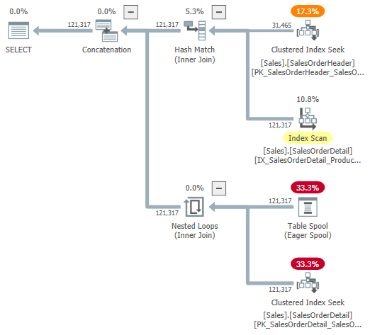
This is a useful representation to aid understanding, but it isn’t entirely accurate, complete, or consistent. For example, the Table Spool doesn’t exist—it’s a default representation for the adaptive buffer reader reading rows directly from the batch mode hash table.

The operator properties and cardinality estimates are also a bit all over the place. The output from the adaptive buffer reader (“spool”) should be 31,465 rows, not 121,317. The subtree cost of the apply is incorrectly capped by the parent operator cost. This is normal for showplan, but it makes no sense in an adaptive join context.

There are other inconsistencies as well—too many to usefully list— but that can happen with undocumented trace flags. The expanded plan shown above isn’t intended for use by end users, so perhaps it isn’t entirely surprising. The message here is not to rely too heavily on the numbers and properties shown in this undocumented form.

I should also mention in passing the finished standard adaptive join plan operator isn’t entirely without its own consistency issues. These stem pretty much exclusively from the hidden details.

For example, the displayed adaptive join properties come from a mixture of the underlying Concat, Hash Join, and Apply operators. You can see an adaptive join reporting batch mode execution for nested loops join (which is impossible), and the elapsed time shown is actually copied from the hidden Concat, not the particular join that executed at runtime.

The Usual Suspects

We can get some useful information from the sorts of undocumented trace flags normally used to look at optimizer output. For example:

SELECT SOH.SubTotal
FROM Sales.SalesOrderHeader AS SOH
JOIN Sales.SalesOrderDetail AS SOD
    ON SOD.SalesOrderID = SOH.SalesOrderID
WHERE SOH.SalesOrderID <= 75123
OPTION (
    QUERYTRACEON 3604,
    QUERYTRACEON 8607,
    QUERYTRACEON 8612);

Output (heavily edited for readability):

This gives some insight into the estimated costs for the full-cardinality case with hash and apply alternatives without writing separate queries and using hints. As mentioned in the main text, these trace flags aren’t effective within CuNewJoinEstimate, so we can’t directly see the repeat calculations for the 31,465-row case or any of the details for the one-row estimates this way.

Merge Join and Row Mode Hash Join

Adaptive joins only offer a transition from batch mode hash join to row mode apply. For the reasons why row mode hash join isn’t supported, see the Intelligent Query Processing Q&A in the Related Reading section. In short, it’s thought row mode hash joins would be too prone to performance regressions.

Switching to a row mode merge join would be another option, but the optimizer doesn’t currently consider this. As I understand it, it’s unlikely to be expanded in this direction in future.

Some of the considerations are the same as they are for row mode hash join. In addition, merge join plans tend to be less easily interchangeable with hash join, even if we limit ourselves to indexed merge join (no explicit sort).

There’s also a much greater distinction between hash and apply than there is between hash and merge. Both hash and merge are suitable for larger inputs, and apply is better suited to a smaller driving input. Merge join isn’t as easily parallelized as hash join and doesn’t scale as well with increasing thread counts.

Given the motivation for adaptive joins is to cope better with significantly varying input sizes—and only hash join supports batch mode processing—the choice of batch hash versus row apply is the more natural one. Finally, having three adaptive join choices would significantly complicate the threshold calculation for potentially little gain.