Cardinality Estimation for a Predicate on a COUNT Expression

This article looks into selectivity and cardinality estimation for predicates on COUNT(*) expressions, as may be seen in HAVING clauses. The details are hopefully interesting in themselves. They also provide an insight into some of the general approaches and algorithms used by the cardinality estimator.

A simple example using the AdventureWorks sample database:

SELECT A.City
  FROM Person.[Address] AS A
  GROUP BY A.City
  HAVING COUNT_BIG(*) = 1;

We are interested in seeing how SQL Server derives an estimate for the predicate on the count expression in the HAVING clause.

Of course the HAVING clause is just syntax sugar. We could equally have written the query using a derived table, or common table-expression:

-- Derived table
SELECT SQ1.City
FROM
(
    SELECT A.City, Expr1001 = COUNT_BIG(*)
    FROM Person.[Address] AS A
    GROUP BY A.City
) AS SQ1
WHERE SQ1.Expr1001 = 1;

-- CTE
WITH Grouped AS
(
    SELECT A.City, Expr1001 = COUNT_BIG(*)
    FROM Person.[Address] AS A
    GROUP BY A.City
)
SELECT G.City
FROM Grouped AS G
WHERE G.Expr1001 = 1;

All three query forms produce the same execution plan, with identical query plan hash values.

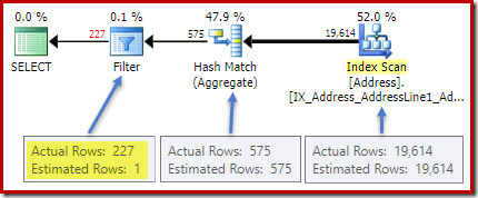
The post-execution (actual) plan shows a perfect estimation for the aggregate; however, the estimate for the HAVING clause filter (or equivalent, in the other query forms) is poor:

Statistics on the City column provide accurate information about the number of distinct city values:

DBCC SHOW_STATISTICS ([Person.Address], City) WITH DENSITY_VECTOR;

The all density figure is the reciprocal of the number of unique values. Simply calculating (1 / 0.00173913) = 575 gives the cardinality estimate for the aggregate. Grouping by city obviously produces one row for each distinct value.

Note that all density comes from the density vector. Be careful not to accidentally use the density value from the statistics header output of DBCC SHOW_STATISTICS. The header density is maintained only for backward compatibility; it is not used by the optimizer during cardinality estimation these days.

The Problem

The aggregate introduces a new computed column to the workflow, labelled Expr1001 in the execution plan. It contains the value of COUNT(*) in each grouped output row:

There is obviously no statistical information in the database about this new computed column. While the optimizer knows there will be 575 rows, it knows nothing about the distribution of count values within those rows.

Well not quite nothing: The optimizer is aware that the count values will be positive integers (1, 2, 3…). Still, it is the distribution of these integer count values among the 575 rows that would be needed to accurately estimate the selectivity of the COUNT(*) = 1 predicate.

One might think that some sort of distribution information could be derived from the histogram, but the histogram only provides specific count information (in EQ_ROWS) for histogram step values. Between histogram steps, all we have is a summary: RANGE_ROWS rows have DISTINCT_RANGE_ROWS distinct values. For tables that are large enough that we care about the quality of the selectivity estimate, it is very likely that most of the table is represented by these intra-step summaries.

For example, the first two rows of the City column histogram are:

DBCC SHOW_STATISTICS ([Person.Address], City) WITH HISTOGRAM;

This tells us that there is exactly one row for "Abingdon", and 29 other rows after "Abingdon" but before "Ballard", with 19 distinct values in that 29-row range. The following query shows the actual distribution of rows among unique values in that 29-row intra-step range:

SELECT A.City, NumRows = COUNT_BIG(*)
FROM Person.[Address] AS A 
WHERE A.City > N'Abingdon' 
AND A.City < N'Ballard'
GROUP BY ROLLUP (A.City);

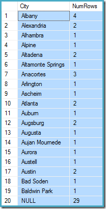
There are 29 rows with 19 distinct values, just as the histogram said. Still, it is clear we have no basis to evaluate the selectivity of a predicate on the count column in that query. For example, HAVING COUNT_BIG(*) = 2 would return 5 rows (for Alexandria, Altadena, Atlanta, Augsburg, and Austin) but we have no way to determine that from the histogram.

An Educated Guess

The approach SQL Server takes is to assume that each group is most likely to contain the overall mean (average) number of rows. This is simply the cardinality divided by the number of unique values. For example, for 1000 rows with 20 unique values, SQL Server would assume that (1000 / 20) = 50 rows per group is the most likely value.

Turning back to our original example, this means that the computed count column is "most likely" to contain a value around (19614 / 575) ~= 34.1113. Since density is the reciprocal of the number of unique values, we can also express that as cardinality * density = (19614 * 0.00173913), giving a very similar result.

Distribution

Saying that the mean value is most likely only takes us so far. We also need to establish exactly how likely that is; and how the likelihood changes as we move away from the mean value. Assuming that all groups have exactly 34.113 rows in our example would not be a very "educated" guess!

SQL Server handles this by assuming a normal distribution. This has the characteristic bell shape you may already be familiar with (image from the linked Wikipedia entry):

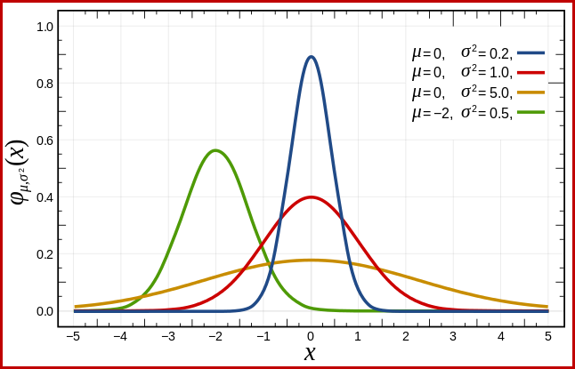
The exact shape of the normal distribution depends on two parameters: the mean (µ) and the standard deviation (σ). The mean determines the location of the peak. The standard deviation specifies how "flattened" the bell curve is. The flatter the curve, the lower the peak is, and the more the probability density is distributed over other values.

SQL Server can derive the mean from statistical information as already noted. The standard deviation of the computed count column values is unknown. SQL Server estimates it as the square root of the mean (with a slight adjustment detailed later on). In our example, this means the two parameters of the normal distribution are roughly 34.1113 and 5.84 (the square root).

The standard normal distribution (the red curve in the diagram above) is a noteworthy special case. This occurs when the mean is zero, and the standard deviation is 1. Any normal distribution can be transformed to the standard normal distribution by subtracting the mean and dividing by the standard deviation.

Areas and Intervals

We are interested in estimating selectivity, so we are looking for the probability that the count computed column has a certain value (x). This probability is given not by the y-axis value above, but by the area under the curve to the left of x.

For the normal distribution with mean 34.1113 and standard deviation 5.84, the area under the curve to the left of x = 30 is about 0.2406:

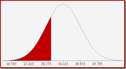
This corresponds to the probability that the computed count column is less than or equal to 30 for our example query.

This leads nicely on to the idea that in general, we are not looking for the probability of a specific value, but for an interval. To find the probably that the count equals an integer value, we need to account for the fact that integers span an interval of size 1. How we convert an integer to an interval is somewhat arbitrary. SQL Server handles this by adding and subtracting 0.5 to give the lower and upper bounds of the interval.

For example, to find the probability that the computed count value equals 30, we need to subtract the area under the normal distribution curve for (x = 29.5) from the area for (x = 30.5). The result corresponds to the slice for (29.5 < x <= 30.5) in the diagram below:

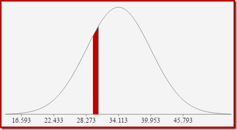
The area of the red slice is about 0.0533. To a good first approximation, this is the selectivity of a count = 30 predicate in our test query.

The Cumulative Distribution Function

Calculating the area under a normal distribution to the left of a given value is not straightforward. The general formula is given by the cumulative distribution function (CDF). The problem is that the CDF cannot be expressed in terms of elementary mathematical functions, so numerical approximation methods have to be used instead.

Since all normal distributions can be easily transformed to the standard normal distribution (mean = 0, standard deviation = 1), the approximations all work to estimate the standard normal. This means we need to transform our interval boundaries from the particular normal distribution appropriate to the query, to the standard normal distribution. This is done, as mentioned earlier, by subtracting the mean and dividing by the standard deviation.

If you are familiar with Excel, you might be aware of the functions NORM.DIST and NORM.S.DIST which can compute CDFs (using numerical approximation methods) for a particular normal distribution or the standard normal distribution.

There is no CDF calculator built in to SQL Server, but we can easily make one. Given that the CDF for the standard normal distribution is:

…where erf is the error function:

A T-SQL implementation to obtain the CDF for the standard normal distribution is shown below. It uses a numerical approximation for the error function that is very close to the one SQL Server uses internally:

CREATE PROCEDURE dbo.GetStandardNormalCDF
(
    @x float,
    @cdf float OUTPUT
)
AS
BEGIN
    SET NOCOUNT, XACT_ABORT ON;
    DECLARE
        @sign float,
        @erf float;
    
    SET @sign = SIGN(@x);
    SET @x = ABS(@x) / SQRT(2);
    SET @erf = 1;
    SET @erf = @erf + (0.0705230784 * @x);
    SET @erf = @erf + (0.0422820123 * POWER(@x, 2));
    SET @erf = @erf + (0.0092705272 * POWER(@x, 3));
    SET @erf = @erf + (0.0001520143 * POWER(@x, 4));
    SET @erf = @erf + (0.0002765672 * POWER(@x, 5)); 
    SET @erf = @erf + (0.0000430638 * POWER(@x, 6));
    SET @erf = POWER(@erf, -16);
    SET @erf = 1 - @erf;
    SET @erf = @erf * @sign;
    SET @cdf = 0.5 * (1 + @erf);
END;

An example, to compute the CDF for x = 30 using the normal distribution for our test query:

DECLARE @cdf float;
DECLARE @x float;
-- HAVING COUNT_BIG(*) = x
SET @x = 30;
-- Normalize 30 by subtracting the mean
-- and dividing by the standard deviation
SET @x = (@x - 34.1113) / 5.84;
EXECUTE dbo.GetStandardNormalCDF
    @x = @x,
    @cdf = @cdf OUTPUT;
SELECT CDF = @cdf;

Note the normalization step to convert to the standard normal distribution. The procedure returns the value 0.2407196…, which matches the corresponding Excel result to seven decimal places.

Final Details and Examples

The following code modifies our example query to produce a larger estimate for the Filter (the comparison is now with the value 32, which is much closer to the mean than before):

SELECT A.City
FROM Person.[Address] AS A
GROUP BY A.City
HAVING COUNT_BIG(*) = 32;

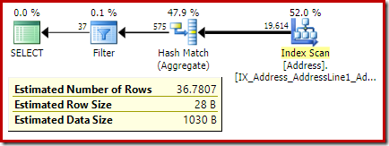
The estimate from the optimizer is now 36.7807.

To compute the estimate manually, we first need to address a few final details:

• The mean used to derive the standard deviation (via square root) is scaled by a factor of ((distinct values – 1) / (distinct values). In the example, the number of distinct values is 575, so the scaling factor is (574 / 575) ~= 0.99826.
• If the lower bound of the (integer) interval is 1, SQL Server treats the interval as unbounded on the lower side. Selectivity is equal to the CDF of the upper bound of the interval (1.5) alone. The lower bound (which would be 0.5) is not used.
• The legacy cardinality estimator (CE) has complex logic for COUNT(*) = 1, which is not detailed here.
• Aside from the COUNT(*) = 1 case, the legacy CE uses the same logic as the new CE (available in SQL Server 2014 onward).

The following procedure incorporates all the details in this article. It requires the CDF procedure given earlier:

CREATE PROCEDURE dbo.GetCountPredicateEstimate
(
    @From           integer,
    @To             integer,
    @Cardinality    float,
    @Density        float,
    @Selectivity    float OUTPUT,
    @Estimate       float OUTPUT
)
AS
BEGIN
    SET NOCOUNT, XACT_ABORT ON;
    BEGIN TRY
    DECLARE
        @Start          float,
        @End            float,
        @Distinct       float,
        @Mean           float,
        @MeanAdj        float,
        @Stdev          float,
        @NormStart      float,
        @NormEnd        float,
        @CDFStart       float,
        @CDFEnd         float;
    -- Validate input and apply defaults
    IF ISNULL(@From, 0) = 0 SET @From = 1;
    IF @From < 1 RAISERROR ('@From must be >= 1', 16, 1);
    IF ISNULL(@Cardinality, -1) <= 0 RAISERROR('@Cardinality must be positive', 16, 1);
    IF ISNULL(@Density, -1) <= 0 RAISERROR('@Density must be positive', 16, 1);
    IF ISNULL(@To, 0) = 0 SET @To = CEILING(1 / @Density);
    IF @To < @From RAISERROR('@To must be >= @From', 16, 1);
    -- Convert integer range to interval
    SET @Start = @From - 0.5;
    SET @End = @To + 0.5;
    -- Get number of distinct values
    SET @Distinct = 1 / @Density;
    -- Calculate mean
    SET @Mean = @Cardinality * @Density;
    -- Adjust mean;
    SET @MeanAdj = @Mean * ((@Distinct - 1) / @Distinct);
    -- Get standard deviation (guess)
    SET @Stdev = SQRT(@MeanAdj);
    -- Normalize interval
    SET @NormStart = (@Start - @Mean) / @Stdev;
    SET @NormEnd = (@End - @Mean) / @Stdev;
    -- Calculate CDFs
    EXECUTE dbo.GetStandardNormalCDF
        @x = @NormStart,
        @cdf = @CDFStart OUTPUT;
    
    EXECUTE dbo.GetStandardNormalCDF
        @x = @NormEnd,
        @cdf = @CDFEnd OUTPUT;
    -- Selectivity
    SET @Selectivity =
        CASE
            -- Unbounded start
            WHEN @From = 1 THEN @CDFEnd
            -- Unbounded end
            WHEN @To >= @Distinct THEN 1 - @CDFStart
            -- Normal interval
            ELSE @CDFEnd - @CDFStart
        END;
    -- Return row estimate
    SET @Estimate = @Selectivity * @Distinct;
    END TRY
    BEGIN CATCH
        DECLARE @EM nvarchar(4000) = ERROR_MESSAGE();
        IF @@TRANCOUNT > 0 ROLLBACK TRANSACTION;
        RAISERROR (@EM, 16, 1);
        RETURN;
    END CATCH;
END;

We can now use this procedure to generate an estimate for our new test query:

DECLARE 
    @Selectivity float,
    @Estimate float;
EXECUTE dbo.GetCountPredicateEstimate
    @From = 32,
    @To = 32,
    @Cardinality = 19614,
    @Density = 0.00173913,
    @Selectivity = @Selectivity OUTPUT,
    @Estimate = @Estimate OUTPUT;
SELECT
    Selectivity = @Selectivity,
    Estimate = @Estimate,
    Rounded = ROUND(@Estimate, 4);

The output is:

This compares very well with the optimizer's cardinality estimate of 36.7807.

Inequality interval examples

The procedure can be used for other count intervals aside from equality tests. All that is required is to set the @From and @To parameters to the integer interval boundaries. To specify unbounded, pass zero or NULL as you prefer.

SELECT A.City
FROM Person.[Address] AS A
GROUP BY A.City
HAVING COUNT_BIG(*) < 50;

To use this with our procedure, we set @From = NULL and @To = 49 (because 50 is excluded by less than):

DECLARE 
    @Selectivity float,
    @Estimate float;
EXECUTE dbo.GetCountPredicateEstimate
    @From = NULL,
    @To = 49,
    @Cardinality = 19614,
    @Density = 0.00173913,
    @Selectivity = @Selectivity OUTPUT,
    @Estimate = @Estimate OUTPUT;
SELECT
    Selectivity = @Selectivity,
    Estimate = @Estimate,
    Rounded = ROUND(@Estimate, 4);

The result is 572.5964:

One last example using BETWEEN:

SELECT A.City
FROM Person.[Address] AS A
GROUP BY A.City
HAVING COUNT_BIG(*) BETWEEN 25 AND 30;

The optimizer estimate is

Since BETWEEN is inclusive, we pass the procedure @From = 25 and @To = 30. The result is:

Again, this agrees with the optimizer estimate.