
Optimization Thresholds – Grouping and Aggregating Data, Part 4
This article is the fourth in a series about optimization thresholds. The series covers grouping and aggregating data, explaining the different algorithms that SQL Server can use, and the costing model that helps it choose between the algorithms. In this article I focus on parallelism considerations. I cover the different parallelism strategies that SQL Server can use, the thresholds for choosing between a serial and a parallel plan, and the costing logic that SQL Server applies using a concept called degree of parallelism for costing (DOP for costing).
I’ll continue using the dbo.Orders table in the PerformanceV3 sample database in my examples. Before running the examples in this article, run the following code to drop a couple of unneeded indexes:
DROP INDEX IF EXISTS idx_nc_sid_od_cid        ON dbo.Orders;
DROP INDEX IF EXISTS idx_unc_od_oid_i_cid_eid ON dbo.Orders;
The only two indexes that should be left on this table are idx_cl_od (clustered with orderdate as the key) and PK_Orders (nonclustered with orderid as the key).
Parallelism strategies
Besides needing to choose between various grouping and aggregation strategies (preordered Stream Aggregate, Sort + Stream Aggregate, Hash Aggregate), SQL Server also needs to choose whether to go with a serial or a parallel plan. In fact, it can choose between multiple different parallelism strategies. SQL Server uses costing logic that results in optimization thresholds that under different conditions make one strategy preferred to the others. We’ve already discussed in depth the costing logic that SQL Server uses in serial plans in the previous parts of the series. In this section I’ll introduce a number of parallelism strategies that SQL Server can use for handling grouping and aggregation. Initially, I won’t get into the details of the costing logic, rather just describe the available options. Later in the article I’ll explain how the costing formulas work, and an important factor in those formulas called DOP for costing.
As you will later learn, SQL Server takes into account the number of logical CPUs in the machine in its costing formulas for parallel plans. In my examples, unless I say otherwise, I assume the target system has 8 logical CPUs. If you want to try out the examples that I’ll provide, in order to get the same plans and costing values like I do, you need to run the code on a machine with 8 logical CPUs as well. If you’re machine happens to have a different number of CPUs, you can emulate a machine with 8 CPUs—for costing purposes—like so:
DBCC OPTIMIZER_WHATIF(CPUs, 8);
Even though this tool is not officially documented and supported, it’s quite convenient for research and learning purposes.
The Orders table in our sample database has 1,000,000 rows with order IDs in the range 1 through 1,000,000. To demonstrate three different parallelism strategies for grouping and aggregation, I’ll filter orders where the order ID is greater than or equal to 300001 (700,000 matches), and group the data in three different ways (by custid [20,000 groups before filtering], by empid [500 groups], and by shipperid [5 groups]), and compute the count of orders per group.
Use the following code to create indexes to support the grouped queries:
CREATE INDEX idx_oid_i_eid ON dbo.Orders(orderid) INCLUDE(empid);
CREATE INDEX idx_oid_i_sid ON dbo.Orders(orderid) INCLUDE(shipperid);
CREATE INDEX idx_oid_i_cid ON dbo.Orders(orderid) INCLUDE(custid);
The following queries implement the aforementioned filtering and grouping:
-- Query 1: Serial

SELECT custid, COUNT(*) AS numorders
FROM dbo.Orders
WHERE orderid >= 300001
GROUP BY custid
OPTION(MAXDOP 1);

-- Query 2: Parallel, not local/global

SELECT custid, COUNT(*) AS numorders
FROM dbo.Orders
WHERE orderid >= 300001
GROUP BY custid;

-- Query 3: Local parallel global parallel

SELECT empid, COUNT(*) AS numorders
FROM dbo.Orders
WHERE orderid >= 300001
GROUP BY empid;

-- Query 4: Local parallel global serial

SELECT shipperid, COUNT(*) AS numorders
FROM dbo.Orders
WHERE orderid >= 300001
GROUP BY shipperid;
Notice that Query 1 and Query 2 are the same (both group by custid), only the former forces a serial plan and the latter gets a parallel plan on a machine with 8 CPUs. I use these two examples to compare the serial and parallel strategies for the same query.
Figure 1 shows the estimated plans for all four queries:
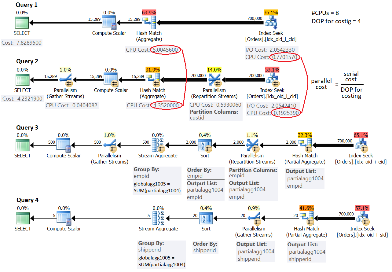 Figure 1: Parallelism strategies
For now, don’t worry about the cost values shown in the figure and the mention of the term DOP for costing. I’ll get to those later. First, focus on understanding the strategies and the differences between them.
The strategy used in the serial plan for Query 1 should be familiar to you from the previous parts in the series. The plan filters the relevant orders using a seek in the covering index you created earlier. Then, with the estimated number of rows to be grouped and aggregated, the optimizer prefers the Hash Aggregate strategy to the Sort + Stream Aggregate strategy.
The plan for Query 2 uses a simple parallelism strategy that employs only one aggregate operator. A parallel Index Seek operator distributes packets of rows to the different threads in a round-robin fashion. Each packet of rows can contain multiple distinct customer IDs. In order for a single aggregate operator to be able to compute the correct final group counts, all rows that belong to the same group must be handled by the same thread. For this reason, a Parallelism (Repartition Streams) exchange operator is used to repartition the streams by the grouping set (custid). Finally, a Parallelism (Gather Streams) exchange operator is used to gather the streams from the multiple threads into a single stream of result rows.
The plans for Query 3 and Query 4 employ a more complex parallelism strategy. The plans start similar to the plan for Query 2 where a parallel Index Seek operator distributes packets of rows to different threads. Then the aggregation work is done in two steps: one aggregate operator locally groups and aggregates the rows of the current thread (notice the partialagg1004 result member), and a second aggregate operator globally groups and aggregates the results of the local aggregates (notice the globalagg1005 result member). Each of the two aggregate steps—local and global—can use any of the aggregate algorithms I described earlier in the series. Both plans for Query 3 and Query 4 start with a local Hash Aggregate and proceed with a global Sort + Stream Aggregate. The difference between the two is that the former uses parallelism in both steps (hence a Repartition Streams exchange is used between the two and a Gather Streams exchange after the global aggregate), and the later handles the local aggregate in a parallel zone and the global aggregate in a serial zone (hence a Gather Streams exchange is used between the two).
When doing your research about query optimization in general, and parallelism specifically, it’s good to be familiar with tools that enable you to control various optimization aspects to see their effects. You already know how to force a serial plan (with a MAXDOP 1 hint), and how to emulate an environment that, for costing purposes, has a certain number of logical CPUs (DBCC OPTIMIZER_WHATIF, with the CPUs option). Another handy tool is the query hint ENABLE_PARALLEL_PLAN_PREFERENCE (introduced in SQL Server 2016 SP1 CU2), which maximizes parallelism. What I mean by this is that if a parallel plan is supported for the query, parallelism will be preferred in all parts of the plan that can be handled in parallel, as if it was free. For instance, observe in Figure 1 that by default the plan for Query 4 handles the local aggregate in a serial zone and the global aggregate in a parallel zone. Here’s the same query, only this time with the ENABLE_PARALLEL_PLAN_PREFERENCE query hint applied (we’ll call it Query 5):
SELECT shipperid, COUNT(*) AS numorders
FROM dbo.Orders
WHERE orderid >= 300001
GROUP BY shipperid
OPTION(USE HINT('ENABLE_PARALLEL_PLAN_PREFERENCE'));
The plan for Query 5 is shown in Figure 2:
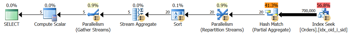 Figure 2: Maximizing parallelism
Observe that this time both the local and the global aggregates are handled in parallel zones.
Serial / parallel plan choice
Recall that during query optimization, SQL Server creates multiple candidate plans and picks the one with the lowest cost among the ones that it produced. The term cost is a bit of a misnomer since the candidate plan with the lowest cost is supposed to be, according to the estimates, the one with the lowest run time, not the one with the lowest amount of resources used overall. For instance, between a serial candidate plan and a parallel one produced for the same query, the parallel plan will likely use more resources, since it needs to use exchange operators that synchronize the threads (distribute, repartition and gather streams). However, in order for the parallel plan to need less time to complete running than the serial plan, the savings achieved by doing the work with multiple threads needs to outweigh the extra work done by the exchange operators. And this needs to be reflected by the costing formulas SQL Server uses when parallelism is involved. Not a simple task to do accurately!
In addition to the parallel plan cost needing to be lower than the serial plan cost in order to be preferred, the cost of the serial plan alternative needs to be greater than or equal to the cost threshold for parallelism. This is a server configuration option set to 5 by default that prevents queries with a fairly low cost to be handled with parallelism. The thinking here is that a system with a large number of small queries would overall benefit more from using serial plans, instead of wasting a lot of resources on synchronizing threads. You can still have multiple queries with serial plans executing at the same time, efficiently utilizing the machine’s multi-CPU resources. In fact, many SQL Server professionals like to increase the cost threshold for parallelism from its default of 5 to a higher value. A system running a fairly small number of large queries simultaneously would benefit much more from using parallel plans.
To recap, in order for SQL Server to prefer a parallel plan to the serial alternative, the serial plan cost needs to be at least the cost threshold for parallelism, and the parallel plan cost needs to be lower than the serial plan cost (implying potentially lower run time).
Before I get to the details of the actual costing formulas, I’ll illustrate with examples different scenarios where a choice is made between serial and parallel plans. Make sure that your system assumes 8 logical CPUs to get query costs similar to mine if you want to try out the examples.
Consider the following queries (we’ll call them Query 6 and Query 7):
-- Query 6: Serial

SELECT empid, COUNT(*) AS numorders
FROM dbo.Orders
WHERE orderid >= 400001
GROUP BY empid;

-- Query 7: Forced parallel

SELECT empid, COUNT(*) AS numorders
FROM dbo.Orders
WHERE orderid >= 400001
GROUP BY empid
OPTION(USE HINT('ENABLE_PARALLEL_PLAN_PREFERENCE'));
The plans for these queries are shown in Figure 3.
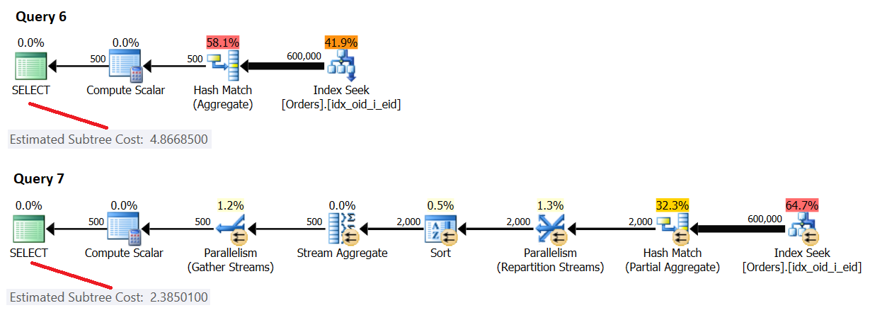 Figure 3: Serial cost < cost threshold for parallelism, parallel cost < serial cost
Here, the [forced] parallel plan cost is lower than the serial plan cost; however, the serial plan cost is lower than the default cost threshold for parallelism of 5, hence SQL Server chose the serial plan by default.
Consider the following queries (we’ll call them Query 8 and Query 9):
-- Query 8: Parallel

SELECT empid, COUNT(*) AS numorders
FROM dbo.Orders
WHERE orderid >= 300001
GROUP BY empid;

-- Query 9: Forced serial

SELECT empid, COUNT(*) AS numorders
FROM dbo.Orders
WHERE orderid >= 300001
GROUP BY empid
OPTION(MAXDOP 1);
The plans for these queries are shown in Figure 4.
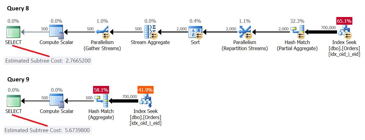 Figure 4: Serial cost >= cost threshold for parallelism, parallel cost < serial cost
Here, the [forced] serial plan cost is greater than or equal to the cost threshold for parallelism, and the parallel plan cost is lower than the serial plan cost, hence SQL Server chose the parallel plan by default.
Consider the following queries (we’ll call them Query 10 and Query 11):
-- Query 10: Serial

SELECT *
FROM dbo.Orders
WHERE orderid >= 100000;

-- Query 11: Forced parallel

SELECT *
FROM dbo.Orders
WHERE orderid >= 100000
OPTION(USE HINT('ENABLE_PARALLEL_PLAN_PREFERENCE'));
The plans for these queries are shown in Figure 5.
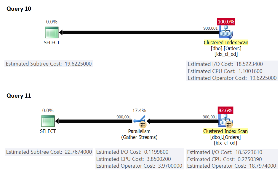 Figure 5: Serial cost >= cost threshold for parallelism, parallel cost >= serial cost
Here, the serial plan cost is greater than or equal to the cost threshold for parallelism; however, the serial plan cost is lower than the [forced] parallel plan cost, hence SQL Server chose the serial plan by default.
There’s another thing that you need to know about attempting to maximize parallelism with the ENABLE_PARALLEL_PLAN_PREFERENCE hint. In order for SQL Server to even be able to use a parallel plan, there has to be some parallelism enabler like a residual predicate, a sort, an aggregate, and so on. A plan that applies just an index scan or index seek without a residual predicate, and without any other parallelism enabler, will be processed with a serial plan. Consider the following queries as an example (we’ll call them Query 12 and Query 13):
-- Query 12

SELECT *
FROM dbo.Orders
OPTION(USE HINT('ENABLE_PARALLEL_PLAN_PREFERENCE'));

-- Query 13

SELECT *
FROM dbo.Orders
WHERE orderid >= 100000
OPTION(USE HINT('ENABLE_PARALLEL_PLAN_PREFERENCE'));
The plans for these queries are shown in Figure 6.
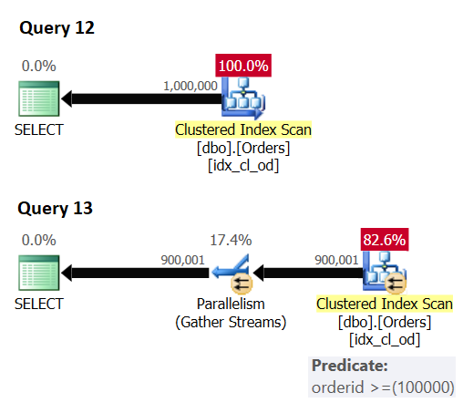 Figure 6: Parallelism enabler
Query 12 gets a serial plan despite the hint since there's no parallelism enabler. Query 13 gets a parallel plan since there's a residual predicate involved.
Computing and testing DOP for costing
Microsoft had to calibrate the costing formulas in an attempt to have a lower parallel plan cost than the serial plan cost reflect a lower run time and vice versa. One potential idea was to take the serial operator’s CPU cost and simply divide it by the number of logical CPUs in the machine to produce the parallel operator’s CPU cost. The logical number of CPUs in the machine is the main factor determining the query’s degree of parallelism, or DOP in short (the number of threads that can be used in a parallel zone in the plan). The simplistic thinking here is that if an operator takes T time units to complete when using one thread, and the query’s degree of parallelism is D, it would take the operator T/D time to complete when using D threads. In practice, things are not that simple. For instance, usually you have multiple queries running simultaneously and not just one, in which case a single query will not get all of the machine’s CPU resources. So, Microsoft came up with the idea of degree of parallelism for costing (DOP for costing, in short). This measure is typically lower than the number of logical CPUs in the machine and is the factor that the serial operator’s CPU cost is divided by to compute the parallel operator’s CPU cost.
Normally, DOP for costing is computed as the number of logical CPUs divided by 2, using integer division. There are exceptions, though. When the number of CPUs is 2 or 3, DOP for costing is set to 2. With 4 or more CPUs, DOP for costing is set to #CPUs / 2, again, using integer division. That’s up to a certain maximum, which depends on the amount of memory available to the machine. In a machine with up to 4,096 MB of memory the maximum DOP for costing is 8; with more than 4,096 MB, maximum DOP for costing is 32.
To test this logic, you already know how to emulate a desired number of logical CPUs using DBCC OPTIMIZER_WHATIF, with the CPUs option, like so:
DBCC OPTIMIZER_WHATIF(CPUs, 8);
Using the same command with the MemoryMBs option, you can emulate a desired amount of memory in MBs, like so:
DBCC OPTIMIZER_WHATIF(MemoryMBs, 16384);
Use the following code to check the existing status of the emulated options:
DBCC TRACEON(3604);

DBCC OPTIMIZER_WHATIF(Status);

DBCC TRACEOFF(3604);
Use the following code to reset all options:
DBCC OPTIMIZER_WHATIF(ResetAll);
Here’s a T-SQL query that you can use to compute DOP for costing based on an input number of logical CPUs and amount of memory:
DECLARE @NumCPUs AS INT = 8, @MemoryMBs AS INT = 16384;

SELECT
  CASE
    WHEN @NumCPUs  = 1 THEN 1
    WHEN @NumCPUs <= 3 THEN 2
    WHEN @NumCPUs >= 4 THEN
      (SELECT MIN(n)
       FROM ( VALUES(@NumCPUs / 2), (MaxDOP4C ) ) AS D2(n))
  END AS DOP4C
FROM ( VALUES( CASE WHEN @MemoryMBs <= 4096 THEN 8 ELSE 32 END ) ) AS D1(MaxDOP4C);
With the specified input values, this query returns 4.
Table 1 details the DOP for costing that you get based on the logical number of CPUs and amount of memory in your machine.
| #CPUs | DOP for costing when MemoryMBs <= 4096 | DOP for costing when MemoryMBs > 4096 |
|---|---|---|
| 1 | 1 | 1 |
| 2-5 | 2 | 2 |
| 6-7 | 3 | 3 |
| 8-9 | 4 | 4 |
| 10-11 | 5 | 5 |
| 12-13 | 6 | 6 |
| 14-15 | 7 | 7 |
| 16-17 | 8 | 8 |
| 18-19 | 8 | 9 |
| 20-21 | 8 | 10 |
| 22-23 | 8 | 11 |
| 24-25 | 8 | 12 |
| 26-27 | 8 | 13 |
| 28-29 | 8 | 14 |
| 30-31 | 8 | 15 |
| 32-33 | 8 | 16 |
| 34-35 | 8 | 17 |
| 36-37 | 8 | 18 |
| 38-39 | 8 | 19 |
| 40-41 | 8 | 20 |
| 42-43 | 8 | 21 |
| 44-45 | 8 | 22 |
| 46-47 | 8 | 23 |
| 48-49 | 8 | 24 |
| 50-51 | 8 | 25 |
| 52-53 | 8 | 26 |
| 54-55 | 8 | 27 |
| 56-57 | 8 | 28 |
| 58-59 | 8 | 29 |
| 60-61 | 8 | 30 |
| 62-63 | 8 | 31 |
| >= 64 | 8 | 32 |
Table 1: DOP for costing
As an example, let’s revisit Query 1 and Query 2 shown earlier:
-- Query 1: Forced serial

SELECT custid, COUNT(*) AS numorders
FROM dbo.Orders
WHERE orderid >= 300001
GROUP BY custid
OPTION(MAXDOP 1);

-- Query 2: Naturally parallel

SELECT custid, COUNT(*) AS numorders
FROM dbo.Orders
WHERE orderid >= 300001
GROUP BY custid;
The plans for these queries are shown in Figure 7.
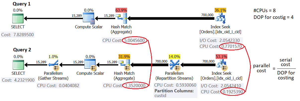 Figure 7: DOP for costing
Query 1 forces a serial plan, whereas Query 2 gets a parallel plan in my environment (emulating 8 logical CPUs and 16,384 MB of memory). This means that DOP for costing in my environment is 4. As mentioned, a parallel operator’s CPU cost is computed as the serial operator’s CPU cost divided by DOP for costing. You can see that that’s indeed the case in our parallel plan with the Index Seek and Hash Aggregate operators which execute in parallel.
As for the costs of the exchange operators, they’re made of a startup cost and some constant cost per row, which you can easily reverse engineer.
Notice that in the simple parallel grouping and aggregation strategy, which is the one used here, the cardinality estimates in the serial and parallel plans are the same. That’s because only one aggregate operator is employed. Later you will see that things are different when using the local/global strategy.
The following queries help illustrate the effect of the number of logical CPUs and number of rows involved on the query cost (10 queries, with increments of 100K rows):
SELECT empid, COUNT(*) AS numorders
FROM dbo.Orders
WHERE orderid >= 900001
GROUP BY empid;

SELECT empid, COUNT(*) AS numorders
FROM dbo.Orders
WHERE orderid >= 800001
GROUP BY empid;

SELECT empid, COUNT(*) AS numorders
FROM dbo.Orders
WHERE orderid >= 700001
GROUP BY empid;

SELECT empid, COUNT(*) AS numorders
FROM dbo.Orders
WHERE orderid >= 600001
GROUP BY empid;

SELECT empid, COUNT(*) AS numorders
FROM dbo.Orders
WHERE orderid >= 500001
GROUP BY empid;

SELECT empid, COUNT(*) AS numorders
FROM dbo.Orders
WHERE orderid >= 400001
GROUP BY empid;

SELECT empid, COUNT(*) AS numorders
FROM dbo.Orders
WHERE orderid >= 300001
GROUP BY empid;

SELECT empid, COUNT(*) AS numorders
FROM dbo.Orders
WHERE orderid >= 200001
GROUP BY empid;

SELECT empid, COUNT(*) AS numorders
FROM dbo.Orders
WHERE orderid >= 100001
GROUP BY empid;

SELECT empid, COUNT(*) AS numorders
FROM dbo.Orders
WHERE orderid >= 000001
GROUP BY empid;
Figure 8 shows the results.
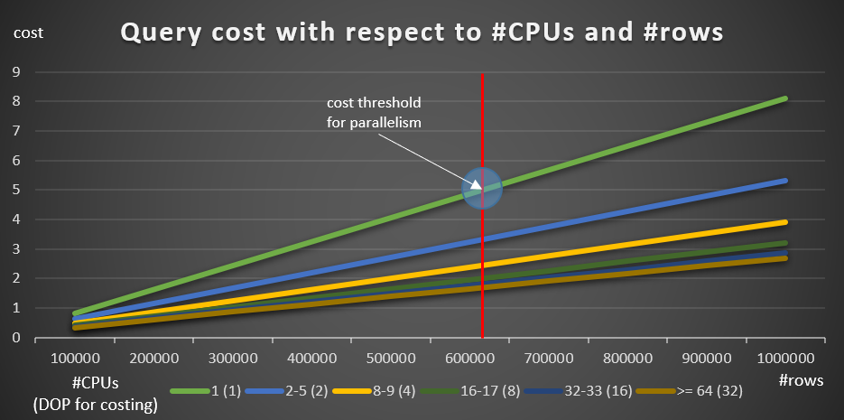 Figure 8: Query cost with respect to #CPUs and #rows
The green line represents the costs of the different queries (with the different numbers of rows) using a serial plan. The other lines represent the costs of the parallel plans with different numbers of logical CPUs, and their respective DOP for costing. The red line represents the point where the serial query cost is 5—the default cost threshold for parallelism setting. To the left of this point (fewer rows to be grouped and aggregated), normally, the optimizer will not consider a parallel plan. In order to be able to research the costs of parallel plans below the cost threshold for parallelism, you can do one of two things. One option is to use the query hint ENABLE_PARALLEL_PLAN_PREFERENCE, but as a reminder, this option maximizes parallelism as opposed to just forcing it. If that’s not the desired effect, you could just disable the cost threshold for parallelism, like so:
EXEC sp_configure 'show advanced options', 1;
RECONFIGURE;

EXEC sp_configure 'cost threshold for parallelism', 0;

EXEC sp_configure 'show advanced options', 0;
RECONFIGURE;
Obviously, that’s not a smart move in a production system, but perfectly useful for research purposes. That’s what I did to produce the information for the chart in Figure 8.
Starting with 100K rows, and adding 100K increments, all graphs seem to imply that had cost threshold for parallelism wasn’t a factor, a parallel plan would have always been preferred. That’s indeed the case with our queries and the numbers of rows involved. However, try smaller numbers of rows, starting with 10K and increasing by 10K increments using the following five queries (again, keep cost threshold for parallelism disabled for now):
SELECT empid, COUNT(*) AS numorders
FROM dbo.Orders
WHERE orderid >= 990001
GROUP BY empid;

SELECT empid, COUNT(*) AS numorders
FROM dbo.Orders
WHERE orderid >= 980001
GROUP BY empid;

SELECT empid, COUNT(*) AS numorders
FROM dbo.Orders
WHERE orderid >= 970001
GROUP BY empid;

SELECT empid, COUNT(*) AS numorders
FROM dbo.Orders
WHERE orderid >= 960001
GROUP BY empid;

SELECT empid, COUNT(*) AS numorders
FROM dbo.Orders
WHERE orderid >= 950001
GROUP BY empid;
Figure 9 shows the query costs with both serial and parallel plans (emulating 4 CPUs, DOP for costing 2).
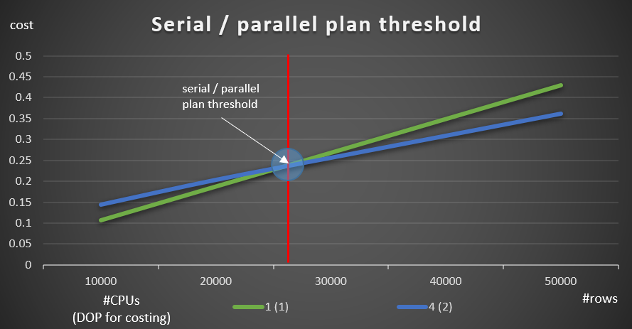 Figure 9: Serial / parallel plan threshold
As you can see, there’s an optimization threshold up to which the serial plan is preferred, and above which the parallel plan is preferred. As mentioned, in a normal system where you either keep the cost threshold for parallelism setting at the default value of 5, or higher, the effective threshold is anyway higher than in this graph.
Earlier I mentioned that when SQL Server chooses the simple grouping and aggregation parallelism strategy, the cardinality estimates of the serial and parallel plans are the same. The question is, how does SQL Server handle the cardinality estimates for the local/global parallelism strategy.
To figure this out, I’ll use Query 3 and Query 4 from our earlier examples:
-- Query 3: Local parallel global parallel

SELECT empid, COUNT(*) AS numorders
FROM dbo.Orders
WHERE orderid >= 300001
GROUP BY empid;

-- Query 4: Local parallel global serial

SELECT shipperid, COUNT(*) AS numorders
FROM dbo.Orders
WHERE orderid >= 300001
GROUP BY shipperid;
In a system with 8 logical CPUs and an effective DOP for costing value of 4, I got the plans shown in Figure 10.
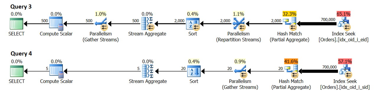 Figure 10: Cardinality estimate
Query 3 groups the orders by empid. 500 distinct employee groups are expected eventually.
Query 4 groups the orders by shipperid. 5 distinct shipper groups are expected eventually.
Curiously, it seems that the cardinality estimate for the number of groups produced by the local aggregate is { number of distinct groups expected by each thread } * { DOP for costing }. In practice, you realize that the number will usually by twice as much since what counts is the DOP for execution (aka, just DOP), which is based primarily on the number of logical CPUs. This part is a bit tricky to emulate for research purposes since the DBCC OPTIMIZER_WHATIF command with the CPUs option affects the computation of DOP for costing, but DOP for execution will not be greater than the actual number of logical CPUs that your SQL Server instance sees. This number is essentially based on the number of schedulers SQL Server starts with. You can control the number of schedulers SQL Server starts with using the -P{ #schedulers } startup parameter, but that’s a bit more aggressive research tool compared to a session option.
At any rate, without emulating any resources, my test machine has 4 logical CPUs, resulting in DOP for costing 2, and DOP for execution 4. In my environment, the local aggregate in the plan for Query 3 shows an estimate of 1,000 result groups (500 x 2), and an actual of 2,000 (500 x 4). Similarly, the local aggregate in the plan for Query 4 shows an estimate of 10 result groups (5 x 2) and an actual of 20 (5 x 4).
When you’re done experimenting, run the following code for cleanup:
-- Set cost threshold for parallelism to default

EXEC sp_configure 'show advanced options', 1;
RECONFIGURE;

EXEC sp_configure 'cost threshold for parallelism', 5;

EXEC sp_configure 'show advanced options', 0;
RECONFIGURE;
GO

-- Reset OPTIMIZER_WHATIF options

DBCC OPTIMIZER_WHATIF(ResetAll);

-- Drop indexes

DROP INDEX idx_oid_i_sid ON dbo.Orders;
DROP INDEX idx_oid_i_eid ON dbo.Orders;
DROP INDEX idx_oid_i_cid ON dbo.Orders;
Conclusion
In this article I described a number of parallelism strategies that SQL Server uses to handle grouping and aggregation. An important concept to understand in the optimization of queries with parallel plans is the degree of parallelism (DOP) for costing. I showed a number of optimization thresholds, including a threshold between serial and parallel plans, and the setting cost threshold for parallelism. Most of the concepts I described here are not unique to grouping and aggregation, rather are just as applicable for parallel plan considerations in SQL Server in general. Next month I’ll continue the series by discussing optimization with query rewrites.
7 thoughts on “Optimization Thresholds – Grouping and Aggregating Data, Part 4”
Comments are closed.
Thanks for the very detailed and easy-to-follow post, i found this incredibly helpful! I'm running into an interesting issue during SQL Server 2014-to-SQL Server 2016 upgrade testing. Many of our queries that have a parallel plan in SS2014 (compatibility level 120) are regressing to much slower serial plans in SS2016 (compatibility level 130). Following the examples from your blog post, I am unable to determine why the plans are now serial.
I have a SQL Server Central post with details on the issue here: https://www.sqlservercentral.com/Forums/1977590/Upgrade-to-Compatibility-Level-130-from-120-Causing-Parallel-Plans-to-Become-Slower-Serial-Plans?Update=1#bm1977749
If you are able, do you mind taking a look at the post and let me know if you have any suggestions? Thanks again!
Hi Chris,
This is indeed strange. I was easily able to reproduce your situation with a simple data warehouse query involving a columnstore index. Also in my case, the chosen serial plan had a higher cost than the [forced] parallel plan. The optimization of the serial plan in compatibility level 130+ terminated early due to a Time Out, and used batch processing (new capability with serial plans in 2016, BTW).
I sent this along with the link to your post to Microsoft, and they said they're looking into this. They also cautioned that the hint to maximize parallelism is undocumented, doesn't always do what people think it does, lacks sufficient testing coverage, and comes with no guarantees. At the same time, they acknowledge the need for a solution in this space, saying they're exploring options.
Cheers,
Itzik
Thanks Itzik, much appreciated. We also opened a support ticket about this issue with MS the other day – we'll update our ticket to mention that you have also contacted them about this. And I'll post updates/solutions here as I get them from MS.
Hi Itzik,
We received a pretty disappointing response from MS support today. Here is their response:
"When you upgrade your database to SQL Server 2016, there will be no plan changes seen if you remain at the older compatibility levels that you were using (for example, 120 or 110). New features and improvements related to query optimizer, will be available only under latest compatibility level.
Therefore, the behavior you’re experiencing is expected and under compatibility level 130 with the new query optimizer. This document has all the information regarding those changes to the query optimizer.
If serial plan is not the ideal option then you’ll need to use the workaround which will be either to:
1. Lower the database compatibility level to 120.
2. Add OPTION(USE HINT('ENABLE_PARALLEL_PLAN_PREFERENCE')) to all affected queries.
3. Enable Trace Flag 8649 to force parallelism"
Options #2 and #3 don't seem to be viable production solutions, and #1 negates the reason for the upgrade in the first place… We'll continue to push back to see if they can provide another solution.
Hi Chris,
I guess this new capability of batch processing in serial plans can potentially improve performance in many cases. What's probably happening in yours is that when the optimizer explores candidate plans, it now has more options to choose from, with the new candidate plans having a low enough cost, that the optimizer decides not to proceed to evaluating the parallel option.
I hear you. It's a bummer that in your case you see a big performance difference compared to the old plans, and that the options provided to you are not very appealing.
Itzik
Hi Itzik,
Have you heard any updates on this from Microsoft or come across a resolution in subsequent CUs or versions of SQL Server?
Thanks,
Mitch
Hi Mitch,
In case you're referring to the issue Chris raised, than no; nothing new beyond what Chris and I already mentioned.