

An important part of query tuning is understanding the algorithms that are available to the optimizer to handle various query constructs, e.g., filtering, joining, grouping and aggregating, and how they scale. This knowledge helps you prepare an optimal physical environment for your queries, such as creating the right indexes. It also helps you intuitively sense which algorithm you should expect to see in the plan under a certain set of circumstances, based on your familiarity with the thresholds where the optimizer should switch from one algorithm to another. Then, when tuning bad performing queries, you can more easily spot areas in the query plan where the optimizer may have made suboptimal choices, for instance due to inaccurate cardinality estimates, and take action to fix those.
Another important part of query tuning is thinking out of the box — beyond the algorithms that are available to the optimizer when using the obvious tools. Be creative. Say you have a query that performs badly even though you arranged the optimal physical environment. For the query constructs that you used, the algorithms available to the optimizer are x, y, and z, and the optimizer chose the best that it could under the circumstances. Still, the query performs badly. Can you imagine a theoretical plan with an algorithm that can yield a much better performing query? If you can imagine it, chances are that you will be able to achieve it with some query rewrite, perhaps with less obvious query constructs for the task.
In this series of articles, I focus on grouping and aggregating data. I’ll start by going over the algorithms that are available to the optimizer when using grouped queries. I’ll then describe scenarios where none of the existing algorithms do well and show query rewrites that do result in excellent performance and scaling.
I’d like to thank Craig Freedman, Vassilis Papadimos, and Joe Sack, members of the intersection of the set of smartest people on the planet and the set of SQL Server developers, for answering my questions about query optimization!
For sample data I’ll use a database called PerformanceV3. You can download a script to create and populate the database from here. I’ll use a table called dbo.Orders, which is populated with 1,000,000 rows. This table has a couple of indexes that are not needed and could interfere with my examples, so run the following code to drop those unneeded indexes:
DROP INDEX idx_nc_sid_od_cid ON dbo.Orders;
DROP INDEX idx_unc_od_oid_i_cid_eid ON dbo.Orders;
The only two indexes left on this table are a clustered index called idx_cl_od on the orderdate column, and a nonclustered unique index called PK_Orders on the orderid column, enforcing the primary key constraint.
EXEC sys.sp_helpindex 'dbo.Orders';
index_name   index_description                                      index_keys
-----------  -----------------------------------------------------  -----------
idx_cl_od    clustered located on PRIMARY                           orderdate
PK_Orders    nonclustered, unique, primary key located on PRIMARY   orderid
Existing algorithms
SQL Server supports two main algorithms for aggregating data: Stream Aggregate and Hash Aggregate. With grouped queries, the Stream Aggregate algorithm requires the data to be ordered by the grouped columns, so you need to distinguish between two cases. One is a preordered Stream Aggregate, e.g., when data is obtained preordered from an index. Another is a nonpreordered Stream Aggregate, where an extra step is required to explicitly sort the input. These two cases scale very differently so you might as well consider them as two different algorithms.
The Hash Aggregate algorithm organizes the groups and their aggregates in a hash table. It does not require the input to be ordered.
With enough data, the optimizer considers parallelizing the work, applying what’s known as a local-global aggregate. In such a case, the input is split into multiple threads, and each thread applies one of the aforementioned algorithms to locally aggregate its subset of rows. A global aggregate then uses one of the aforementioned algorithms to aggregate the results of the local aggregates.
In this article I focus on the preordered Stream Aggregate algorithm and its scaling. In future parts of this series I will cover other algorithms and describe the thresholds where the optimizer switches from one to another, and when you should consider query rewrites.
Preordered Stream Aggregate
Given a grouped query with a nonempty grouping set (the set of expressions that you group by), the Stream Aggregate algorithm requires the input rows to be ordered by the expressions forming the grouping set. When the algorithm processes the first row in a group, it initializes a member holding the intermediate aggregate value with the relevant value (e.g., first row’s value for a MAX aggregate). When it processes a nonfirst row in the group, it assigns that member with the result of a computation involving the intermediate aggregate value and the new row’s value (e.g., the maximum between the intermediate aggregate value and the new value). As soon as any of the grouping set’s members changes its value, or the input is consumed, the current aggregate value is considered to be the final result for the last group.
One way to have the data ordered like the Stream Aggregate algorithm needs is to obtain it preordered from an index. You need the index to be defined with the grouping set’s columns as the keys—in any order among them. You also want the index to be covering. For example, consider the following query (we’ll call it Query 1):
SELECT shipperid, MAX(orderdate) AS maxorderid
  FROM dbo.Orders
  GROUP BY shipperid;
An optimal rowstore index to support this query would be one defined with shipperid as the leading key column, and orderdate either as an included column, or as a second key column:
CREATE INDEX idx_sid_od ON dbo.Orders(shipperid, orderdate);
With this index in place, you get the estimated plan shown in Figure 1 (using SentryOne Plan Explorer).
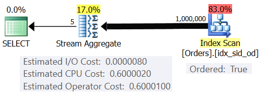
Figure 1: Plan for Query 1
Notice that the Index Scan operator has an Ordered: True property signifying that it is required to deliver the rows ordered by the index key. The Stream Aggregate operator then ingests the rows ordered like it needs. As for how the operator’s cost is computed; before we get to that, a quick preface first…
As you may already know, when SQL Server optimizes a query, it evaluates multiple candidate plans, and eventually picks the one with the lowest estimated cost. The estimated plan cost is the sum of all the operators’ estimated costs. In turn, each operator’s estimated cost is the sum of the estimated I/O cost and estimated CPU cost. The cost unit is meaningless in its own right. Its relevance is in the comparison that the optimizer makes between candidate plans. That is, the costing formulas were designed with the goal that, between candidate plans, the one with the lowest cost will (hopefully) represent the one that will finish more quickly. A terribly complex task to do accurately!
The more the costing formulas adequately take into account the factors that truly affect the algorithm’s performance and scaling, the more accurate they are, and the more likely that given accurate cardinality estimates, the optimizer will choose the optimal plan. At any rate, if you want to understand why the optimizer chooses one algorithm versus another you need to understand two main things: one is how the algorithms work and scale, and another is SQL Server’s costing model.
So back to the plan in Figure 1; let’s try and understand how the costs are computed. As a policy, Microsoft will not reveal the internal costing formulas that they use. When I was a kid I was fascinated with taking things apart. Watches, radios, cassette tapes (yes, I’m that old), you name it. I wanted to know how things were made. Similarly, I see value in reverse engineering the formulas since if I manage to predict the cost reasonably accurately, it probably means that I understand the algorithm well. During the process you get to learn a lot.
Our query ingests 1,000,000 rows. Even with this number of rows, the I/O cost seems to be negligible compared to the CPU cost, so it is probably safe to ignore it.
As for the CPU cost, you want to try and figure out which factors affect it and in what way. Theoretically there could be a number of factors: number of input rows, number of groups, cardinality of grouping set, data type and size of grouping set’s members. So, to try and measure the effect of any of these factors, you want to compare estimated costs of two queries that differ only in the factor that you want to measure. For instance, to measure the impact of the number of rows on the cost, have two queries with a different number of input rows, but with all other aspects the same (number of groups, cardinality of grouping set, etc.). Also, it’s important to verify that the estimated numbers—not the actuals—are the desired ones since the optimizer relies on the estimated numbers to compute costs.
When doing such comparisons, it’s good to have techniques that allow you to fully control the estimated numbers. For instance, a simple way to control the estimated number of input rows is to query a table expression that is based on a TOP query and apply the aggregate function in the outer query. If you’re concerned that due to your use of the TOP operator the optimizer will apply row goals, and that those will result in adjustment of the original costs, this only applies to operators that appear in the plan below the Top operator (to the right), not above (to the left). The Stream Aggregate operator naturally appears above the Top operator in the plan since it ingests the filtered rows.
As for controlling the estimated number of output groups, you can do so by using the grouping expression <integercolumn> % <numgroups> (% is T-SQL’s modulo operator). Naturally, you will want to make sure that the distinct number of values in <integercolumn> isn’t smaller than <numgroups>. Also, be aware that this trick doesn’t work with the legacy cardinality estimator. When estimating the cardinality resulting from filtering or grouping based on an expression that manipulates a column, the legacy CE (compatibility 70 through 110) simply always uses the formula SQRT(<input_cardinality>), irrespective of the expression that you used. So for an input with 100,000 rows, the grouping expression gets a cardinality estimate of 316.228 groups. With an input cardinality of 200,000 rows, you get an estimate of 447.214 groups. Fortunately, the new cardinality estimators (compatibility 120 and above) do a much better job in such cases. I’m running my examples on SQL Server 2017 CU 4 (compatibility 140), so as you will see shortly, it’s quite safe to use this trick to control the estimated number of groups. Note that when grouping by an expression you will get an explicit sort preceding the Stream Aggregate operator, but our goal in this exercise is just to figure out how the Stream Aggregate operator’s CPU cost is computed, so we’ll simply ignore all other operators in the plan for now.
To make sure that you get the Stream Aggregate algorithm and a serial plan you can force this with the query hints: OPTION(ORDER GROUP, MAXDOP 1).
You also want to figure out if there’s any startup cost for the operator so that you can take it into account in your reverse engineered formula.
Let’s start by figuring out the way the number of input rows affects the operator’s estimated CPU cost. Clearly, this factor should be relevant to the operator’s cost. Also, you’d expect the cost per row to be constant. Here are a couple of queries for comparison that differ only in the estimated number of input rows (call them Query 2 and Query 3, respectively):
SELECT orderid % 10000 AS grp, MAX(orderdate) AS maxod
  FROM (SELECT TOP (100000) * FROM dbo.Orders) AS D
  GROUP BY orderid % 10000
  OPTION(ORDER GROUP, MAXDOP 1);

SELECT orderid % 10000 AS grp, MAX(orderdate) AS maxod
  FROM (SELECT TOP (200000) * FROM dbo.Orders) AS D
  GROUP BY orderid % 10000
  OPTION(ORDER GROUP, MAXDOP 1);
Figure 2 has the relevant parts of the estimated plans for these queries:
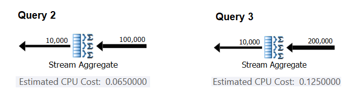
Figure 2: Plans for Query 2 and Query 3
Assuming the cost per row is constant, you can compute it as the difference between the operator costs divided by the difference between the operator input cardinalities:
CPU cost per row = (0.125 - 0.065) / (200000 - 100000) = 0.0000006
To verify that the number you got is indeed constant and correct, you can try and predict the estimated costs in queries with other numbers of input rows. For instance, the predicted cost with 500,000 input rows is:
Cost for 500K input rows = <cost for 100K input rows> + 400000 * 0.0000006 = 0.065 + 0.24 = 0.305
Use the following query to check whether your prediction is accurate (call it Query 4):
SELECT orderid % 10000 AS grp, MAX(orderdate) AS maxod
  FROM (SELECT TOP (500000) * FROM dbo.Orders) AS D
  GROUP BY orderid % 10000
  OPTION(ORDER GROUP, MAXDOP 1);
The relevant part of the plan for this query is shown in Figure 3.
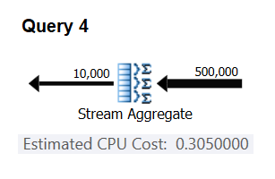
Figure 3: Plan for Query 4
Bingo. Naturally, it’s a good idea to check multiple additional input cardinalities. With all the ones that I checked, the thesis that there’s a constant cost per input row of 0.0000006 was correct.
Next, let’s try and figure out the way the estimated number of groups affects the operator’s CPU cost. You’d expect some CPU work to be needed to process each group, and it’s also reasonable to expect it to be constant per group. To test this thesis and compute the cost per group, you can use the following two queries, which differ only in the number of result groups (call them Query 5 and Query 6, respectively):
SELECT orderid % 10000 AS grp, MAX(orderdate) AS maxod
  FROM (SELECT TOP (100000) * FROM dbo.Orders) AS D
  GROUP BY orderid % 10000
  OPTION(ORDER GROUP, MAXDOP 1);

SELECT orderid % 20000 AS grp, MAX(orderdate) AS maxod
  FROM (SELECT TOP (100000) * FROM dbo.Orders) AS D
  GROUP BY orderid % 20000
  OPTION(ORDER GROUP, MAXDOP 1);
The relevant parts of the estimated query plans are shown in Figure 4.
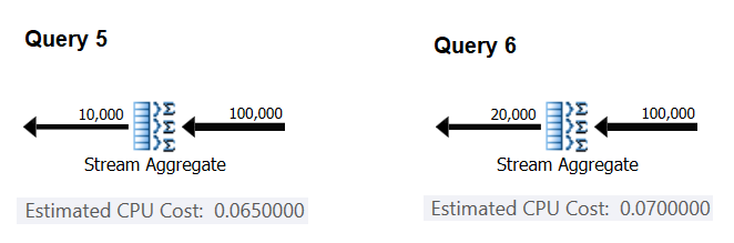
Figure 4: Plans for Query 5 and Query 6
Similar to the way you computed the fixed cost per input row, you can compute the fixed cost per output group as the difference between the operator costs divided by the difference between the operator output cardinalities:
CPU cost per group = (0.07 - 0.065) / (20000 - 10000) = 0.0000005
And just like I demonstrated before, you can verify your findings by predicting the costs with other numbers of output groups and comparing your predicted numbers with the ones produced by the optimizer. With all numbers of groups that I tried, the predicted costs were accurate.
Using similar techniques, you can check if other factors affect the operator’s cost. My testing shows that the cardinality of the grouping set (number of expressions that you group by), the data types and sizes of the grouped expressions have no impact on the estimated cost.
What’s left is to check if there’s any meaningful startup cost assumed for the operator. If there is one, the complete (hopefully) formula to compute the operator’s CPU cost should be:
Operator CPU cost = <startup cost> + <#input rows> * 0.0000006 + <#output groups> * 0.0000005
So you can derive the startup cost from the rest:
Startup cost =- (<#input rows> * 0.0000006 + <#output groups> * 0.0000005)
You could use any query plan from this article for this purpose. For example, using the numbers from the plan for Query 5 shown earlier in Figure 4, you get:
Startup cost = 0.065 - (100000 * 0.0000006 + 10000 * 0.0000005) = 0
As it would appear, the Stream Aggregate operator doesn’t have any CPU-related startup cost, or it’s so low that it isn’t shown with the precision of the cost measure.
In conclusion, the reverse-engineered formula for the Stream Aggregate operator cost is:
I/O cost: negligible
CPU cost: <#input rows> * 0.0000006 + <#output groups> * 0.0000005
Figure 5 depicts the scaling of the Stream Aggregate operator’s cost with respect to both the number of rows and the number of groups.
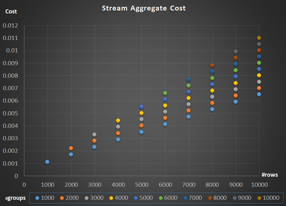
Figure 5: Stream Aggregate algorithm scaling chart
As for the operator’s scaling; it’s linear. In cases where the number of groups tends to be proportional to the number of rows, the entire operator’s cost increases by the same factor that both the number of rows and groups increase. Meaning that doubling the number of both input rows and input groups results in doubling the entire operator’s cost. To see why, suppose that we represent the operator’s cost as:
r * 0.0000006 + g * 0.0000005
If you increase both the number of rows and the number of groups by the same factor p, you get:
pr * 0.0000006 + pg * 0.0000005 = p * (r * 0.0000006 + g * 0.0000005)
So if, for a given number of rows and groups, the cost of the Stream Aggregate operator is C, increasing both the number of rows and groups by the same factor p results in an operator cost of pC. See if you can verify this by identifying examples in the chart in Figure 5.
In cases where the number of groups stays pretty stable even when the number of input rows grows, you still get linear scaling. You just consider the cost associated with the number of groups as a constant. That is, if for a given number of rows and groups the cost of the operator is C = G (cost associated with number of groups) plus R (cost associated with number of rows), increasing just the number of rows by a factor of p results in G + pR. In such a case, naturally, the entire operator’s cost is less than pC. That is, doubling the number of rows results in less than doubling of the entire operator’s cost.
In practice, in many cases when you group data, the number of input rows is substantially larger than the number of output groups. This fact, combined with the fact that the allocated cost per row and cost per group are almost the same, the portion of the operator’s cost that is attributed to the number of groups becomes negligible. As an example, see the plan for Query 1 shown earlier in Figure 1. In such cases, it’s safe to just think of the operator’s cost as simply scaling linearly with respect to the number of input rows.
Special cases
There are special cases where the Stream Aggregate operator doesn’t need the data sorted at all. If you think about it, the Stream Aggregate algorithm has a more relaxed ordering requirement from the input compared to when you need the data ordered for presentation purposes, e.g., when the query has an outer presentation ORDER BY clause. The Stream Aggregate algorithm simply needs all rows from the same group to be ordered together. Take the input set {5, 1, 5, 2, 1, 2}. For presentation ordering purposes, this set has to be ordered like so: 1, 1, 2, 2, 5, 5. For aggregation purposes, the Stream Aggregate algorithm would still work well if the data was arranged in the following order: 5, 5, 1, 1, 2, 2. With this in mind, when you compute a scalar aggregate (query with an aggregate function and no GROUP BY clause), or group the data by an empty grouping set, there’s never more than one group. Irrespective of the order of the input rows, the Stream Aggregate algorithm can be applied. The Hash Aggregate algorithm hashes the data based on the grouping set’s expressions as the inputs, and both with scalar aggregates and with an empty grouping set, there are no inputs to hash by. So, both with scalar aggregates and with aggregates applied to an empty grouping set, the optimizer always uses the Stream Aggregate algorithm, without requiring the data to be preordered. That’s at least the case in row execution mode, since currently (as of SQL Server 2017 CU4) batch mode is available only with the Hash Aggregate algorithm. I’ll use the following two queries to demonstrate this (call them Query 7 and Query 8):
SELECT COUNT(*) AS numrows FROM dbo.Orders;

SELECT COUNT(*) AS numrows FROM dbo.Orders GROUP BY ();
The plans for these queries are shown in Figure 6.
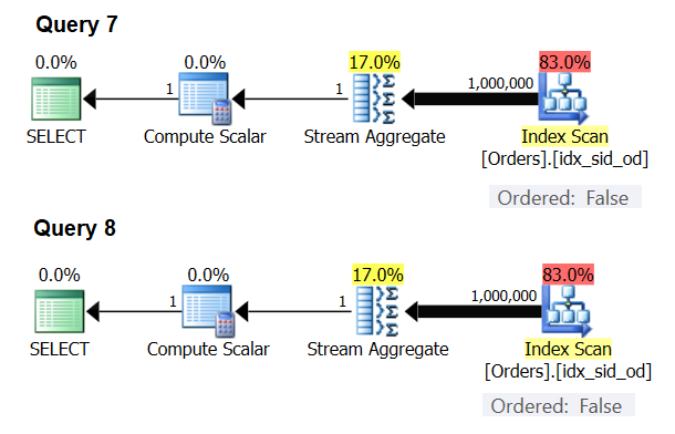
Figure 6: Plans for Query 7 and Query 8
Try forcing a Hash Aggregate algorithm in both cases:
SELECT COUNT(*) AS numrows FROM dbo.Orders OPTION(HASH GROUP);

SELECT COUNT(*) AS numrows FROM dbo.Orders GROUP BY () OPTION(HASH GROUP);
The optimizer ignores your request and produces the same plans shown in Figure 6.
Quick quiz: what’s the difference between a scalar aggregate and an aggregate applied to an empty grouping set?
Answer: with an empty input set, a scalar aggregate returns a result with one row, whereas an aggregate in a query with an empty grouping set returns an empty result set. Try it:
SELECT COUNT(*) AS numrows FROM dbo.Orders WHERE 1 = 2;
numrows
-----------
0

(1 row affected)
SELECT COUNT(*) AS numrows FROM dbo.Orders WHERE 1 = 2 GROUP BY ();
numrows
-----------

(0 rows affected)
When you’re done, run the following code for cleanup:
DROP INDEX idx_sid_od ON dbo.Orders;
Summary and challenge
Reverse-engineering the costing formula for the Stream Aggregate algorithm is a child’s play. I could have just told you that the costing formula for a preordered Stream Aggregate algorithm is @numrows * 0.0000006 + @numgroups * 0.0000005 instead of a whole article to explain how you figure this out. The point, however, was to describe the process and the principles of reverse-engineering, before moving on to the more complex algorithms and the thresholds where one algorithm becomes more optimal than the others. Teaching you how to fish instead of giving you fish kind of thing. I’ve learned so much, and discovered things I haven’t even thought about, while trying to reverse-engineer costing formulas for various algorithms.
Ready to test your skills? Your mission, should you choose to accept it, is a notch more difficult than reverse-engineering the Stream Aggregate operator. Reverse-engineer the costing formula of a serial Sort operator. This is important for our research since a Stream Aggregate algorithm applied for a query with a non-empty grouping set, where the input data is not preordered, requires explicit sorting. In such a case the cost and scaling of the aggregate operation depends on the cost and scaling of the Sort and the Stream Aggregate operators combined.
If you manage to get decently close with predicting the cost of the Sort operator, you can feel like you earned the right to add to your signature “Reverse Engineer.” There are many software engineers out there; but you certainly don’t see many reverse engineers! Just make sure to test your formula both with small numbers and with large ones; you might be surprised by what you find.


"Where's the EASY button?" j/k You're shining a light on a black box for me. Thanks.
Thanks, Chris!
Am so excited for the next part in the series :)
Well, my reverse engineered costing formula for the Sort surprised me! Interested to see what you have to say about this in the next post, particularly to learn the reason why my expectation was wrong.
Fantastic information, as always, Itzik. Lucid, engaging, and deep!
Is there any chance that the PerformanceV3 database is schema-compatible, meaning it uses some or all of the tables, with the sample databases from your books?
Best regards,
-Kev
Thanks, Kevin!
PerformanceV3 is indeed the sample database from my books.